


| Issue |
EPJ Nuclear Sci. Technol.
Volume 12, 2026
|
|
|---|---|---|
| Article Number | 20 | |
| Number of page(s) | 51 | |
| DOI | https://doi.org/10.1051/epjn/2026011 | |
| Published online | 19 June 2026 | |
https://doi.org/10.1051/epjn/2026011
Regular Article
The 0E2 benchmarks for PWR UO2 decay heat: an analysis from the NEA WPNCS
1
Paul Scherrer Institute (PSI), Villigen, Switzerland
2
Centro de Investigaciones Energéticas, Medioambientales y Tecnológicas (CIEMAT), Madrid, Spain
3
OECD Nuclear Energy Agency (NEA), Paris, France
4
JFoster & Associates, LLC (JFA), Idaho Falls, ID, USA
5
Nuclear Safety and Radiation Protection Authority (ASNR), Fontenay-aux-Roses, France
6
Universidad Politécnica de Madrid (UPM), Madrid, Spain
7
Commissariat à l’énergie atomique et aux énergies alternatives (CEA), Cadarache, France
8
Karlsruhe Institute of Technology (KIT), Karlsruhe, Germany
9
Belgian Nuclear Research Centre (SCK CEN), Mol, Belgium
10
Subatech (CNRS/IN2P3, IMT Atlantique, Université de Nantes), Nantes, France
11
ENRESA, Madrid, Spain
12
Gesellschaft für Zwischenlagerung (BGZ), Essen, Germany
13
Bundesamt für die Sicherheit der nuklearen Entsorgung (BASE), Salzgitter, Germany
14
VTT Technical Research Centre of Finland (VTT), Espoo, Finland
15
EPFL, Lausanne, Switzerland
16
Svensk Kärnbränslehantering AB (SKB), Solna, Sweden
17
Jožef Stefan Institute (JSI), Ljubljana, Slovenia
18
Commissariat à l’énergie atomique et aux énergies alternatives (CEA), Saclay, France
19
ORANO, Beaumont Hague, France
20
ORANO, Montigny-le-Bretonneux, France
21
National Nuclear Laboratory (NNL), Seascale, UK
22
Oak Ridge National Laboratory (ORNL), Oak Ridge, TN, USA
23
Central Research Institute of Electric Power Industry (CRIEPI), Nagasaka, Japan
24
Science Engineering Associates, Madrid, Spain
25
Studsvik Scandpower, Inc., Newton, MA, USA
26
Nagra, Wettingen, Switzerland
* e-mail: This email address is being protected from spambots. You need JavaScript enabled to view it.
Received:
11
February
2026
Received in final form:
30
March
2026
Accepted:
8
April
2026
Published online: 19 June 2026
Abstract
This paper presents the work performed in the subgroup 16 of the Working Party for Nuclear Criticality Safety (WPNCS) of the OECD Nuclear Energy Agency. The main goal was to define two decay heat benchmarks for Spent Nuclear Fuel (one pincell and one assembly), perform calculations and compare and analyze the results in light of existing calorimetric measurements. The selected case is the PWR UO2 assembly 0E2, irradiated at the Ringhals-3 reactor and measured at the Clab facility in Sweden. In total, 21 institutes worldwide participated to the exercise, leading to 55 calculated results (named C). It was found that the measured decay heat values (E) can be satisfactorily reproduced with two-dimensional assembly calculations, leading to an average C/E value of 0.99, with an uncertainty (or one standard deviation) of ±0.01.
© D.A. Rochman et al., Published by EDP Sciences, 2026
 This is an Open Access article distributed under the terms of the Creative Commons Attribution License (https://creativecommons.org/licenses/by/4.0), which permits unrestricted use, distribution, and reproduction in any medium, provided the original work is properly cited.
1. Introduction
Decay heat is one of the most relevant quantities for the characterization of spent nuclear fuel (SNF, or UNF for Used Nuclear fuel) when considering interim storage and deep geological repository. Its estimation also impacts the design and operation at reprocessing facilities, SNF transport, safeguard operations and fuel cycle decisions. Maximum values on decay heat can be obtained once thermal limits are known for a given installation, leading to a limit for the number of SNF assemblies at a specific location. Other quantities of high interest include the neutron multiplication factor, the assembly initial material composition, burnup at the end of life, gamma and neutron emission and initial fuel mass. Given the large number of SNF assemblies worldwide, the dependence on decay heat calculation is inevitable, with such estimations possibly being compared to direct measurements in a limited number of cases. A review of the current knowledge on SNF decay heat was recently performed at the OECD1 Nuclear Energy Agency by an expert group of the Working Party of Nuclear Criticality Safety (WPNCS), and can be found in reference [1]. The state of the art, at the time of publication, for simulations, theoretical calculations, measurements and standard methods is presented in this reference, leading to a number of recommendations. If the situation regarding calorimetric measurements for assembly decay heat has recently improved with the release of reference [2] in 2024 (the previous reference publication dated from 2006 [3]), sensibly increasing the number of available measurements for validation, previous related experience indicated that a new blind benchmark exercise would provide real value towards improving our computational models, methods, and analyses approaches for decay heat calculation. In such an exercise, participants provide the results of their calculations, which are later compared with undisclosed experimental values of decay heat. The value of this approach is to avoid being influenced by published values, thus reflecting the real-life situation that national experts might encounter. Reference [4] was a first attempt of a blind benchmark for decay heat, including many institutes, using different simulation tools, different nuclear data libraries, and different analysts (called users, or participants). Unfortunately, an unexpected bias in the measurements did not allow to fully take advantage of the effort. Still, the outcome provided valuable information for establishing a more effective benchmark exercise in the future, and calculated data C, compared with experimental values E and with average calculated values indicated tolerance limits of ±5% (with 95% probability that the limits contain 95% of the population) and a standard deviation close to 2%. Alternatively, reference [1] also indicates a 2% standard deviation (Fig. 2 in the reference), but for a set of published C/E values. There are consequently indications that the SNF decay heat, for UO2 fuel, can be estimated globally with a 2% standard deviation. Such results naturally raise other questions, such as their generalization to other cases (different fuel types, initial enrichments, and burnup values), their implications to the estimations of relevant nuclides (relevant for decay heat, but also for criticality-safety), and the extrapolation to 2 or 3 standard deviations to correctly quantify the population of C and C/E values. The current benchmark exercise is not a blind benchmark as previously described, but pursues the very ambitious goal of estimating biases and uncertainties on calculated decay heat, in a case of a SNF assembly with known design and operation history, and decay heat measurements. It contributes to assessing our prediction capabilities, and ultimately our ability to correctly quantify the previously mentioned C/E distribution. As described in the next section, the decay heat of the 0E2 assembly, irradiated at the Pressurized Water Reactor (PWR) Ringhals 3, was measured at the Clab facility [3]. Two benchmarks were defined by the “sub-group 16” (SG16) of the WPNCS (see details in the following), and a number of participants calculated various quantities, among them decay heat values at six cooling times, corresponding to six calorimetric measurements. In addition, other quantities were requested from participants, to help disentangling possible modeling differences. These calculated values will be analyzed in the following. Regarding the decay heat calculations, the results of this study will be presented and analysed as distributions of C/E ratios. As the main results of the present study, the C/E distributions are presented in Figure 1 for both defined benchmarks: the pincell and assembly models.
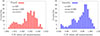 |
Fig. 1. Distributions of the decay heat C/E values for the 6 measurements. Left: pincell benchmark; Right: assembly benchmark. n is the number of C/E values. |
As main conclusions, one can see that the results from the pincell benchmark tend to overestimate the measurements, whereas for the assembly benchmark, the average C/E is close to 1, nonetheless with a spread close to the previously mentioned standard deviations. These values, for the decay heat as well as for nuclide concentrations, reaction rates, k∞ (or neutron multiplication factor in an infinite medium) and decay heat contributions, are analyzed in the present paper. The definition of the benchmarks are first presented in Section 2, followed by the analysis approach (Sect. 3), and the results in Section 4. The main outcomes of the present study are presented in Section 5, followed by the conclusions. Information on specific calculations, tabulated values for averages, standard deviations and tolerance limits are given in the appendices.
2. Definition of benchmarks
The benchmarks used in the SG16 were defined based on the descriptions of the 0E2 assembly from the SKB report R-05-62 [3]. As presented in the following, some additional information are also extracted from references [5, 6]. This PWR assembly was irradiated in Sweden, at the Ringhals 3 reactor, for four consecutive cycles (noted C2 to C5, following the notation from the SKB report), reaching an assembly-average final burnup of 41.6 MWd/kg2. It consists of a 17×17 Westinghouse assembly design, with an initial 235U enrichment of 3.1%.
The benchmarks represent two different systems, both being two-dimensional models: a single pincell from the 0E2 assembly, and the 0E2 assembly itself. In addition, the decay heat rate measurements used in the present work were obtained from the SKB report and reference [7], and represent six experimental values from calorimetric measurements performed at six different cooling times, for the entire three-dimensional assembly. Details are provided in the following sections and the full benchmark descriptions can be found in reference [8].
If the pincell model is a simplistic approximation of the 0E2 assembly and its irradiation, the assembly model is as close to reality as it can be, given the available public information. It is therefore expected the bias between the calculated and measured assembly decay heat will have a reasonably small value. This is supported by recent studies on the 0E2 assembly, for instance in references [5, 7, 9–12], where the considered models of the 0E2 assembly led to acceptable results.
2.1. Assembly model
The description of the 0E2 assembly and its irradiation history are presented in Tables A.1 to A.3. These dimensions correspond to cold conditions and the benchmark does not consider thermal expansion (expected to be negligible for decay heat calculations); references to publications are included. When an information provided in the tables does not originate from a specific reference, a note is added. The assembly average burnup is 41.6 MWd/kg, and the initial enrichment in 235U is 3.1%. The assembly can be modeled using a quarter symmetry, as presented in Figure 2 using CASMO5 and SCALE plots. For the 2D simulation, no modeling for the spacers is required, and no specific material at the top and bottom of the assembly needs to be modeled. The necessary data for creating the assembly model and its irradiation conditions are presented in Appendix A and correspond to reference [8].
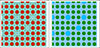 |
Fig. 2. Quarter symmetry representations of the assembly 0E2. Right: CASMO5 plot; Left: SCALE plot. Large blue circles are guide and instrument tubes, whereas green (left) and red (right) circles are UO2 rods. |
2.2. Pincell model
The pincell considered in this exercise corresponds to a UO2 rod from the 0E2 assembly model described in the previous section. The same fuel pellet geometry, initial fuel composition, cladding and irradiation history are to be used for both the assembly and the pincell (see Fig. 3).
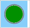 |
Fig. 3. View of pincell benchmark. Colors represent the different zones of UO2 (green), air (white), cladding (gray) and coolant (blue). |
Details of the characteristics of the pincell model can be found in Table A.4 and correspond to reference [8]. The pin geometry data, including the pin pitch, and fuel compositions from the assembly have been kept unchanged for this pincell model, and a reflective boundary condition is applied. Therefore, the moderation ratio (H/M) of this pincell model is different than for the assembly model, leading as expected to different k∞ values (up to 1000 pcm for fresh fuel), 239Pu and minor actinides built-up, and decay heat values.
2.3. Measurements
A total of six measurements were performed for assembly 0E2, using the Clab calorimeter. The first one is mentioned in reference [3], and the five later ones in reference [7]. The measurement data are summarized in Table 1, with the cooling time being expressed as relative to the shutdown date for cycle C5: July 7, 1988.
Reported decay heat rate experimental values for the assembly 0E2.
For all the calorimetric measurements, the contribution from the gamma-ray escape is considered constant and equal to 15.5 W [3]. The values of the total decay heat rate3 (being the sum of the components from the gamma-ray escape and from the calorimeter itself) are considered as reference values in the present study. The total decay heat rate values from Table 1 will be referred to as “E” and the calculated decay heat rate values as “C”.
2.4. Calculated quantities
The main interest of the benchmark resides in the calculation of the decay heat values at the time of the measurements (see Tab. 1). These six decay heat calculated values are therefore required as output of the benchmark (both for the pincell and assembly models):
-
at the six cooling time of measurements, the calculated decay heat values (in Watts),
-
at the six cooling time of measurements, the contributions (in %) to the total decay heat for 238 − 240Pu, 241Am, 244Cm, 90Sr, 90Y, 134, 137Cs, 137mBa and 154Eu.
In addition, in order to help for the understanding of possible spread of results, as well as to estimate possible differences due to the depletion calculations, the following quantities are also requested for both the pincell and the assembly calculations:
-
k∞at the beginning and end of each of the four irradiation cycles,
-
burnup value (MWd/kg) at the beginning and end of each of the four cycles,
-
similarly, mass densities (in g/tHM4) for 234 − 236, 238U, 238 − 242Pu, 241, 242m, 243Am, 242 − 244Cm, 90Sr, 134, 137Cs, 148Nd and 154Eu at the beginning and end of each of the four cycles,
-
the integrated number of fission for 235, 238U and 239, 241Pu (in % of the total fission) at the end of each cycle.
Finally, the neutron and gamma-ray emission rates were also requested at the time of decay heat measurements. In the case of the gamma-ray emission, it was suggested during the SG16 (and not given in the benchmark description [8]) to follow the 7 energy groups (in MeV): [0.5 − 0.7], [0.7 − 1.0], [1.0 − 1.5], [1.5 − 2.0], [2.0 − 2.5], [2.5 − 3.0], and [3.0 − 4.0]. Participants did not systematically provide such information; consequently the neutron and gamma emissions are not analyzed in the present work.
For simplicity, the following notation will be used in tables and in the text:
-
For beginning of life (or irradiation): BOL, with a burnup of 0 MWd/kg.
-
For the end of 1st cycle: EOC2, with a burnup of 7.491 MWd/kg.
-
For the beginning of the 2nd cycle: BOC3, with a burnup of 7.491 MWd/kg.
-
For the end of the 2nd cycle: EOC3, with a burnup of 20.5 MWd/kg.
-
For the end of the 3nd cycle: EOC4, with a burnup of 31.8 MWd/kg.
-
For the end of the 4nd cycle: EOL, with a burnup of 41.6 MWd/kg.
-
For decay heat measurements: DH1 up to DH6.
The notation C2 to C4 refers to the cycle number 2 to 4, as described in the original reference [3]; cycle C2 is the first cycle where the assembly 0E2 was irradiated.
3. Analysis
The main goal of the analysis is to estimate how the current calculations, with model descriptions based on available information, can reproduce high-quality measurements performed on the selected SNF assembly. This study is not a full blind benchmark, as the experimental reference data are already known and available at the time of the study, but results as provided by participants were shared prior to the present analysis.
If the model descriptions are unique, their implementations may vary depending on a number of criteria, such as the considered transport and depletion code, the nuclear data library (both for neutron transport, fuel depletion and decay), and the user’s effect. These three “parameters” (which are here referred to as ULC, U for user, L for Library and C for code) may be the most relevant ones for the estimation of the calculated decay values, and the additional requested quantities, e.g. k∞, nuclide concentrations and reaction rates. These observations on influential parameters are applied for the present analysis, as described in the section devoted to the method (Sect. 3.1).
In support of the present analysis, the SG16 participants have performed calculations for the benchmark cases (both the pincell and the assembly), with the development of their own models, and their choice of codes, nuclear data libraries, and possibly other hidden parameters. A complete list is presented in Table 2. In total, 55 sets of simulations were performed by different users, with a variety of codes and libraries. In this table, “XS” refers to the cross section library, “DD” to the decay data library, and “FY” to the fission yield library.
Description of the options used by participants. “p/a/pa” respectively means pincell, assembly and both pincell and assembly benchmarks. Superscripts are the total calculation cases. A unique value for the library in column 3 indicates that all nuclear data (XS, FY and DD) comes from this library.
As indicated, participants may have performed calculations for the pincell or the assembly only (indicated with the letter “p” or “a” in the table, for the pincell and assembly, respectively). The total numbers for the pincell and assembly models are indicated in brackets in the table: 38 pincell calculations and 43 assembly calculations.
Type of neutron transport and depletion codes and libraries, associated with the model case.
In Table 2, a number (last column) is assigned to each user, allowing to estimate possible cases where one user performed various calculations (either with the same or different codes). This will be useful for the estimation of so-called “unique” cases, which are a list of indices (from the first column of Tab. 2) corresponding to calculations with different ULC parameters (different nuclear data libraries, codes and users, see the section on method for details). Different calculation results were based on different codes or a nuclear data library, as presented in Table 3. In the case of calculations with ORIGAMI (index #45), such results are counted as the ones from ORIGEN, as ORIGAMI uses ORIGEN as a depletion/decay solver. It can be observed that the codes and libraries are not evenly distributed, with a large majority of participants using the neutron transport and depletion code SERPENT, and the ENDF/B-VII.1 library being often selected.
As presented in the following, the large representation of the code SERPENT and of the nuclear data library ENDF/B-VII.1 explain the difference between the calculated quantities called “All” and “ULC” in tables presented in the following. If the ones under the label “All” correspond to the present distributions of results (without any selection or rejection mechanism), the second ones, based on selected cases (see next section), correspond to distributions based on unique codes, libraries, and users. Given this basis of calculations, the method of analysis is then detailed in the next section.
3.1. Method
The present analysis is facing a number of challenges. The first one concerns the large amount of data calculated by each participant. In addition to the six decay heat values, the other calculated quantities are helping to assess the similarities in modeling (for instance at the start of irradiation), and in the depletion process. The second challenge concerns the inputs to the calculations, identified as three main ones: user, library and code. They influence the independence of each calculation, as well as their correlations. It will be important in the following to assess the impact of these three quantities: in a global way, but also individually, if possible. Finally, the last aspect to take into account is the overwhelming number of results based on SERPENT and also on the ENDF/B-VII.1 library (possibly together, but not systematically, see Tab. 3). These characteristics affect statistical quantities such as averages and standard deviations. Each of these points is detailed in the following paragraphs.
3.1.1. Number of output quantities
With more than 160 requested quantities, including nuclide concentrations, k∞, and decay heat contributors, the interpretation of the results will be presented in Section 4 for the most relevant quantities. An emphasis will be placed on reaction rates and k∞ at the beginning of irradiation, where the depletion process does not intervene. Then, the evolution of k∞ with irradiation will also be analyzed as a data set. The main reason is that it has also been studied in numerous other studies, for instance to compare transport and depletion codes [13, 14], or libraries [15]. A third group of data will concern the evolution of nuclide concentrations, which are at the origin of the estimation of the decay heat. The nuclides of interest are of relevance for decay heat, but also for criticality, linking the present work (on decay heat) to criticality aspects. The estimation of nuclide concentrations is also of interest for code validation, as it is usually done with Post Irradiation Examination (PIE) and measurements included in database such as SFCOMPO [16]. Finally, the decay heat values at measured cooling times, their contributors and nuclide concentrations will be analyzed as a fourth category of data.
3.1.2. Disentanglement of the ULC inputs
As previously mentioned, it is assumed that the different calculations performed for both the pincell and assembly cases can be approximated by a function of three different input parameters, shortly named ULC for (1) the user, (2) the nuclear data library, and (3) the transport and depletion code. Each of these input parameters, or variables, is listed in Tables 2 and 3. For a specific calculated output value, e.g. k∞ at the beginning of irradiation (or k∞BOL), different statistical quantities can be obtained (see Sect. 3.2), the most simple being the average or the standard deviation. As an illustration, Figure 4 presents the k∞BOL distribution for the pincell (left) and assembly (right) models, based on all calculations. The following quantities can be extracted (see Tabs. B.1 and B.5 for the complete set of values):
-
Averages:
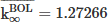 for the pincell model, and 1.28571 for the assembly model.
 -
Standard deviations: 1σ = 482 pcm for the pincell model and 381 pcm for the assembly model (1 pcm =10−5).
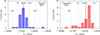 |
Fig. 4. Distribution of the k∞BOL for the pincell (left) and assembly model (right), from all participants (indexed from 1 to 55 from Tab. 2). |
Other statistical quantities can be obtained, but for the sake of simplicity, we will focus only on the average value (mean value) and standard deviation (1σ). These two values are representative of all calculations performed with the current population of cases. But given the repetition of certain inputs (ULC), and the over-representation of some codes and libraries, these average and standard deviation do not represent a population of inputs with equal weights.
It is therefore of interest to also consider distributions not biased towards a specific set of ULC. It is for instance unlikely that future studies based on large numbers of fuel assemblies will be performed with Monte Carlo transport codes (because of the high number of SNF per country, thousands or tens of thousands of spent fuel assemblies), simply due to the large required calculation time. The general use of the ENDF/B-VII.1 library as observed in this work might also not be representative of studies performed in organizations with a strong experience and development in nuclear data libraries. It is possible to estimate the values of  and σ from simulation cases with unique values of ULC; for instance, for the pincell model, one can select from Table 2 the calculations with the indexes 1, 19, 23, 26 and 50, for which the same code, user, or library is not used twice or more. One can also select 1, 3, 12, 14, 16, 20 and 47. For these two cases, one obtains the following values:
-
cases 1, 19, 23, 26, 50:
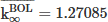 and σ = 411 pcm,
 -
cases 1, 3, 12, 14, 16, 20 and 47:
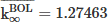 and σ = 871 pcm.
Clearly, these two examples do not lead to similar standard deviations. It is certainly more informative to generalize these two cases by selecting all the possible combinations with unique values of ULC. Given the number of indexes in Table 2, and by randomly searching thousands of times, there is a total of 2364 combinations leading to unique cases of ULC. By taking all of them into account and calculating the averages of  and of σ (among the 2364 ULC k∞BOL values), one obtains 1.27236 and 456 pcm, respectively. These values can be considered as more representative of what would be obtained from independent calculations, without any overlap from similar nuclear data libraries, transport and depletion codes, or users. Consequently, such values from unique ULC will also be reported in the next sections and tables.
Following the same approach, one can also have solely a unique parameter among the ULC (for instance, L), and letting the other ones be freely selected. For instance, if one is interested by repeating the previous example, but considering unique libraries (for instance, with indexes 1, 3, 11, 13, 14, 17, 19, 23, 24, 33 and 49), a total of 9764 combinations is found based on a Monte Carlo combinatorial search. By generalization, the following values summarize the results, in the case of k∞BOL for the pincell model:
-
All calculations (i.e. all indexes):
 pcm;
pcm; -
Unique ULC (2364 combinations):
 pcm;
pcm; -
Unique U (5975 combinations):
 pcm;
pcm; -
Unique L (9764 combinations):
 pcm;
pcm; -
Unique C (3924 combinations):
 pcm.
pcm.
The numbers after the ± sign correspond to the average of the standard deviations. Some remarks can be made based on these quantities. First, the averages are different, but globally within a few hundreds pcm. As there are no measurements to compare to, it can simply be noted that for this k∞ quantity, the value of “unique ULC” is close to the one obtained with a simple average of all data. The one with unique libraries is the most different, indicating the strong impact of nuclear data libraries on the calculation of k∞. Regarding the standard deviations, the one from “unique ULC” is also very similar to the simple average of all results. The three other standard deviations (for unique U, unique L and unique C) help to quantify the impact of the three parameters. For instance, the effect of the nuclear data library is the largest. This is expected, as different cross sections are known to strongly impact criticality values. The effect of different codes is the smallest of the three. This is also an indication that codes similarly handle neutron transport at beginning of life. Finally, the user effect is not negligible. It can for instance influence k∞BOL through different user interpretations of the benchmark description.
In the following, similar decomposition of effects will be presented for other quantities, including for the decay heat C/E values.
3.2. Statistical quantities
As previously mentioned, different distributions can be considered: directly from the simulations, or processed to obtain unique ULC, or unique U, L or C. Each case presents some interests, and they will therefore be presented in the following.
For each distribution, a number of representative quantities will be presented: the average, the standard deviation σ (often interpreted as the uncertainty), and tolerance limits. Other parameters can be calculated, such as the median, the median average deviation, or the confidence on the average. Even if useful, these parameters will not be provided. In the case of the tolerance limits, the case of 95%/95% will be given (95% probability that the limits contain 95% of the population). An example is given in Table 4 for some quantities of the pincell and assembly benchmarks at beginning and end of life. Generally, the values obtained from unique ULC will be the reference values for the analysis.
Example of calculated quantities in the case of the pincell and assembly benchmarks. Values with a ± sign are average ±σ, whereas values within solid brackets ([ ]) are 95%/95% tolerance limits. In bold are indicated the reference values. RR refers to reaction rates (fractions of the total fission rate).
All values presented in the examples will be repeated in the Appendixes, but the main tables inserted in the main text will only include the ULC results.
4. Results
4.1. Beginning of irradiation
The beginning of the 0E2 irradiation is of interest due to the expected agreement between participants’ results. Only a few representative quantities can be analyzed to quantify similarities between the different modeling approaches. As the initial composition of the UO2 fuel is clearly specified in the pincell and assembly benchmarks (being equal to each other), the reported initial concentrations of 234U5, 235U, and 238U are expected to be the same among participants. Similarly, no indication of the presence of 236U was given. Values of interest can be found in Tables B.1 to B.9.
Concerning 235U, and 238U, the reported concentrations are indeed very consistent, with standard deviations smaller than 0.05%. The data provided in Table B.1 for the BOL mass of 235U per MTHM show that the user-applied enrichment for 235U was on average 3.1005%, which differs from the 3.103% value provided in the benchmark, indicating that most of the users did not apply the benchmark-provided value. The standard deviation shown for 235U at BOL seems small in value, however its impact is not trivial on k∞ at BOL. If for the pin cell model, this standard deviation is added to the enrichment value, k∞ varies by ≃120 pcm.
A larger spread for 234U is found (between 1 and 2%), but based on past experience, this is not expected to impact the simulations. The main reason for such changes can be related to default values of 234U added to the initial fuel content by specific codes. Leaving aside 234U, such general agreement will therefore facilitate comparisons for increasing burnup values, understanding that the initial models are highly equivalent from a fuel content aspect.
For 236U, though no indication was given in the benchmark description, different initial concentrations were used by the participants. Most of them used a concentration of zero, and two are equal to 10−13 g/t. High concentrations of 236U can modify the k∞ value, as well as the calculated decay heat (due to a higher build-up of 238Pu). The consistent use of (almost) zero concentration at BOL implies that possible differences in decay heat cannot be attributed to the initial models.
Three other quantities were requested at BOC: k∞, as well as the fission rates from 235U and 238U (named RR). Given that the initial fuel contents are on average similar between participants, deviations in these three quantities would likely reflect differences in the geometrical models (User effect), or in the transport calculations (Library and Code effects). Values of interest are presented in Table 4 (and in the appendix). The uncertainty (1σ) on k∞ is 456 pcm and 371 pcm in the pin and assembly benchmarks for unique ULC, which is larger than the value of 300 pcm reported in reference [17] for another PWR assembly depletion benchmark exercise. Figure 4 presents the distribution of k∞ at BOL for both benchmarks and all provided participants contributions. One value is beyond 3σ for the pincell benchmark (value from index #3), and removing it brings the standard deviation close to 360 pcm. It is a known deficiency of the standard deviation to be sensitive to extreme values, making it sensitive to individual values for small populations. One can also note that the effect of the nuclear data library uncertainty was estimated about 600 pcm to 900 pcm for LCT benchmarks6, being thermal systems, with lattice of UO2 fuel pins, similar to the 0E2 assembly [19, 20]. These values are close to the one for the pincell benchmark and unique libraries (700 pcm). The tolerance limits are nevertheless indicating a large spread, due to very different minimum and maximum as indicated in Figure 4 for the pincell model.
Regarding the fission rates, average values also differ, but uncertainties are very similar in absolute terms. The origin of these differences in terms of fission rates can lie in the values of recoverable fission energy, which might be code specific.
Given the values of Table 4 and the expected differences based on the mentioned references, it is concluded that the simulations of the BOC are similar enough between participants; next burnup steps are then analyzed, keeping in mind the mentioned minimal differences at BOC.
4.2. Neutron multiplication factor k∞
The comparison of the evolution with burnup of k∞ is part of for the present analysis. All burnup steps and cooling time between cycles are fixed by the benchmark definitions and k∞ values were requested at different burnup points. The spread of the results, in terms of one standard deviation, is presented in Table 5, in pcm and in percentage.
Calculated k∞ standard deviations based the ULC approach.
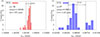 |
Fig. 5. Distributions of the k∞BOL (left) and k∞EOL (right) for the assembly benchmark, from all participants (indexed from 1 to 55). |
These values correspond to the ULC calculations, i.e. excluding all repetitions in the inputs (users, libraries and codes). All other values are presented in Table B.1 of the appendix (for the BOC and EOC, Fig. 5 presents the histograms of the k∞ distributions for the assembly benchmark, for all individual participant contributions). The main trend is the increase of the widths of the distributions with increased burnup values. This increase is more pronounced in the case of the assembly, compared to the pin case. It can be noted that the propagation of nuclear data uncertainties usually do not indicate an increase in k∞ uncertainties (mainly due to the fact that the uncertainties due to 235U are generally larger than the ones from 239Pu [20]); the present observation might therefore not be correlated with the effect of nuclear data. One can also observe that the distributions seem to significantly deviate from Normal distributions, which modifies our usual understanding of a standard deviation. In the present cases, one standard deviation does not represent 68% of the population.
In Figure 5, one can observe the spread at the BOL and EOL, with the same x-scale in both parts of the figure. Three groups of trends can roughly be observed at EOL, and the tendencies are emphasized in Figure 6 as a function of the burnup values. In this figure, the curves are colored to differentiate the calculations based on SERPENT, MCNP (corresponding to MCNP, EVOLCODE and ALEPH) and “other codes" (e.g. Polaris, DARWIN, SNF). Points represents the average differences of k∞ at specific burnup steps for the group considered. The three groups were created by grouping calculations leading to similar results. They are not systematically clearly separated, as there are some overlaps, but different directions between the MCNP and SERPENT calculations can still be seen. If the first code does not present a strong change of slopes for increasing burnup values, results from SERPENT does, with an inflection point close to mid-EOL burnup.
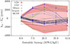 |
Fig. 6. Evolution of k∞ (relative to the average |

Calculated 148Nd (in g/t) in the case of the pincell and assembly benchmarks. Only direct (named “All”) and ULC values are presented here, and other values can be found in Appendix B.
Such separation is not seen if one differentiates nuclear data libraries or users. In summary, in addition to an increase of spread of k∞ values with increasing burnup, the code effects seem to lead to different k∞ trends.
Regarding the different uncertainties obtained considering unique sets of inputs (U, L, and C) or not, variations as a function of burnup are globally similar, with some specific local changes (see Tab. B.1). At EOL, the standard deviations from unique users (U) and unique libraries (L) are nevertheless more important than the one from unique codes (C). This might be not surprising in the case of nuclear data, as it was already observed in a number of publications, but the present study also points out that the choices made by the analysts (users) are not without consequences.
4.3. Concentration of 148Nd
The evolution of the concentration of 148Nd as a function of the pincell or assembly burnup is of high importance, not only with respect to the decay heat calculations. 148Nd is considered as a burnup indicator, as its build-up during irradiation is experimentally quasi linearly increasing. This nuclide production mainly depends on fission yields of 235U and 239Pu (with second order effects from the fission yields of 238U and 241Pu and the 147Nd(n,γ) cross section) [21].
Similarly, the calculated concentration increase is therefore almost linear, and this characteristics is expected from each of the cases of Table 2. The calculated averages and standard deviations are presented in Table 6 (see also B.34 and B.35), and the evolution of the 148Nd concentration is presented in Figure 7, relative to the average values, given in %.
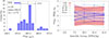 |
Fig. 7. Left: Distribution of the 148NdEOL nuclide concentration for the assembly benchmark. Right: Evolution of 148Nd (relative to the average concentration) as a function of burnup for the assembly benchmark. |
One can see that the uncertainty is relatively flat with burnup, with one standard deviation being close to 1%. The ULC standard deviations seem to be systematically higher than the values directly obtained from the data, but remaining in the vicinity of 1%. Two standard deviations cover most of the cases. The second observation is that most of the calculated trends are linear with burnup, and one can see two exceptions.
The first one (case 23) is showing a strong change of gradient, which is not expected for the usual 148Nd build-up. The library and code used in this case are also similar to other cases, maybe except for the coupling between the transport and depletion calculations. The second case (number 42) is showing the lowest value at EOL (2% from the average). This trend is in fact shared between all cases 37 to 42, and case 42 is the most pronounced one. As many nuclear data libraries are varied from case 37 to 42, the observed difference is likely to originate from the user or code effect.
Spreads of calculated 148Nd were also observed in the literature. Reference [4] indicates a standard deviation of 1.6% for the decay heat blind benchmark, whereas in reference [17], one finds 1%. In addition, an analysis of the uncertainties due to nuclear data and other operating parameters [22–24] presents calculated standard deviations on 148Nd ranging from 0.5 to 1%, depending on assumptions and nuclear data libraries. Another important quantity for the evolution of the 148Nd and its comparison between different simulations is the fission Q-value. This quantity can vary between simulation codes and also nuclear data libraries [25], and affect the evolution of the 148Nd as a function of the pincell or assembly burnup. The standard deviation obtained in the present analysis is therefore in agreement with the literature results.
Calculated 235U (in g/t) in the case of the pincell and assembly benchmarks. Only direct (named “All”) and ULC values are presented here, and other values can be found in Appendix B.
Calculated 239Pu (in g/t) in the case of the pincell and assembly benchmarks. Only direct (named “All”) and ULC values are presented here, and other values can be found in Appendix B.
Based on the present results, one should not expect the precision of the calculations to be better than 1 to 2% for 148Nd concentrations. The effect of nuclear data (148Nd originates from both the fission of 235U and 239Pu, with possible compensations due to variations of fission yields), depletion codes (with possible different recoverable energies per fission) and users can certainly lead to such spread of results, even for fixed burnup values.
4.4. Concentrations of 235U and 239Pu
The two nuclides 235U and 239Pu evolutions with burnup are also of prime interest for the depletion calculation. Their estimations can impact any quantities during, or at the end of the irradiation, such as nuclide concentrations, decay heat, and neutron multiplication factor.
235U is naturally being depleted during irradiation, mainly through fission reactions, and 239Pu is primarily built-up through neutron captures on 238U, partially compensated by its own neutron capture and fission. The concentration of these nuclides can therefore vary for different nuclear data libraries, codes (for instance with different Q-values, fission energy release and deposition models) and benchmark models (e.g. with slightly different water to fuel ratios). The summary for the different concentrations for these nuclides is presented in Tables 7 and 8, with details in Appendix B. As mentioned in Section 4.1, the initial concentration of 235U is not exactly the same for all participants, with small variations for both the pincell and assembly models. Regarding the ULC values, uncertainties are generally slightly smaller than in the case of direct calculations from the raw distributions. Changes are nevertheless not significant compared to the amplitude of average concentrations.
Additionally, differences appear for these concentrations between the pincell and assembly models, implying a lower 235U fission rate in the pincell model, and more 239Pu build-up also in the pincell model (the neutron spectrum is more thermal in the assembly case). As indicated for the analysis of the decay heat values, different actinide concentrations lead in the present case to similar decay heat values. This can be expected, as the decay heat contribution from these two nuclides is minor, but it also indicates that different criticality values (about 600–800 pcm difference between the pincell and the assembly models) and different fissioning actinides can be obtained, while having similar decay heat values. In the case of the assembly model, the distributions for these nuclides at EOL are presented in Figure 8 (left part), with the variations of the distributions as a function of the assembly burnup (right part). For both nuclides, values outside the two sigma bands can be observed (with non-monotonic changes in the case of 235U, as indicated in green in the figure), but the main feature is the increase of the uncertainty for the 235U concentrations and relatively stable values for 239Pu. As mentioned above, these behaviors do not strongly affect the decay heat values, given that compensations can appear for the production of fission products between these two actinides. On the contrary, such spread of concentrations for these two key actinides can impact criticality calculations. Uncertainties of 1.8% and 2.7%, as presented in Figure 8 would significantly affect k∞ or k eff values for SNF criticality models. For comparison, uncertainties due to nuclear data, as presented in Section 4.2 range between 1 and 4% for these nuclides. In summary, such concentrations cannot be assumed to be perfectly known, and uncertainties (as one standard deviation) for SNF shall not be assumed lower than 2%.
In combination with the distributions of these two important nuclide concentrations, it is also of relevance to associate these conclusions with the ones from the fission rates. This is presented in the next section.
4.5. Fission rates
Fission rates are directly linked to the nuclide concentrations, but as the burnup values for both the pincell and assembly benchmarks are fixed, the recoverable energies calculated or used by the depletion codes are also influencing quantities. In the present calculations, fission rates were provided by participants for four nuclides: 235, 238U and 239, 241Pu. They are expected to cover most of the fission rates, and the sum of their contributions is normalized to 100% (values can be found in Tabs. B.10 to B.13).
At the BOL, only two nuclides contribute to the fission rates: 235U and 238U. The differences among participants in the concentrations for these two nuclides are relatively small, in the order of 0.02 to 0.05% (1σ) for both the pincell and assembly benchmarks. For the assembly (and the same conclusions can be obtained for the pincell), 235U contributes to about 94% of the total fission rates and 238U fills the remaining 6%. The 1σ uncertainty obtained directly for the values of the participants is for both nuclides 0.2% (or in relative terms 0.2 and 3.2% for both nuclides and the pincell benchmark). This spread is significantly larger than for the initial concentrations and potentially indicates an effect from nuclear data libraries (cross sections, Q-values), possibly in combination with the effect from codes. The ULC analysis indicates that when unique codes are selected, the above uncertainty increases to 0.3% (for the pincell model), pointing to the use of different recoverable energies (given as fixed quantities in the source code).
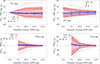 |
Fig. 9. Evolution of reaction rates as a function of burnup for relevant actinides for the assembly benchmark. |
Figure 9 presents the changes of the reaction rates with respect to the burnup and until EOL. As the total of the reaction rates is summing to 100%, the values from the different nuclides are correlated. This can be observed for the highlighted cases. A few cases differ from the general trends: cases 1, 10, 11, 12 and to a lesser extent case 24.
Generally, similar observations can be made for the four considered nuclides: (1) uncertainties are larger for fission rates compared to uncertainties in nuclide concentrations, and (2) the analysis with unique codes also increases the uncertainty on all fission rates. In addition, relatively large variations were observed at EOL for 235U fission rates, with extreme values for the summed contributions larger than 10%.
In conclusion, the above observations indicate that the current burnup calculations are likely affected by different recoverable energies provided by the depletion codes. As shown in Section 4.8 and besides these differences, performing calculations with fixed burnup at EOL leads to similar decay heat values.
4.6. Other nuclide concentrations
Several concentrations for other nuclides were asked from the participants, such as some minor actinides (Pu, Am and Cm) and fission products (Cs, Sr, Eu). The choice of these nuclides was motivated by their effects on the burnup calculations, neutron multiplication values and naturally on decay heat. The most important contributors to the decay heat, for the selected cooling times, were included: 90Sr (its decay 90Y was not requested due to its short half-life and direct proportionality to 90Sr), 137Cs (similarly, 137mBa was also not part of the list of nuclides), 238Pu, 241Am, 244Cm and of less importance: 154Eu and 240Pu. Concerning minor actinides, their burnup evolutions with respect to the calculated average concentrations are presented in Figure 10. Averages and standard deviations can be found in Appendix B. As for the previous figures, standard deviations, in terms of 1 and 2σ, are included, and some outliers (at EOL) are indicated in different colors. Each curve represents the difference with the average concentration for a specific calculation case (from Tab. 9). For these nuclides, it was checked that the indicated trend did not change during the cooling times of interest (for both the individual curve trend and the spread of results). Some remarks are presented in the following, focusing on the impact such evolutions can have on the estimation of decay heat. As mentioned, one of the drawbacks of the standard deviation is that it is sensitive to extreme values (contrary to other quantifiers such as the average deviation or the median average deviation). This can be observed in the figure for nuclides with low concentrations (241Am, and also 241, 243Am and 242Cm not presented in the figure); but due to its common usage, we will continue to present results based on this quantity. Complete distributions should nevertheless be taken into account when available.
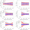 |
Fig. 10. Evolution of concentrations as a function of burnup for minor actinides for the assembly benchmark. |
Fractions to the total decay heat (DH1) at 5823 days, for both benchmarks (average and one standard deviation). Only ULC values are presented, as other analyses lead to similar values.
The concentration of 234U is globally similar for all calculation types (parallel curves as a function of burnup), and the spread is relatively limited. Given that 234U weakly contributes to the decay heat for the cooling time of interest (about 10−2 W/t), it is considered not important for decay heat in the case considered here. It is nevertheless one of the considered actinides for burnup credit, and its concentration is of interest for k∞ calculations. Uncertainties due to nuclear data strongly vary from one library to the other (see values in Ref. [22]: from a few tenths of percent up to 10%), and the standard deviation obtained in the present work is of the same order of magnitude.
In the case of 236U, the concentrations at BOL (before depletion calculations) are zero, as indicated in Section 4.1. Initial concentrations of 236U can impact the amount of 238Pu during cooling; no relevant changes are observed.
238Pu is one of the important contributors to the decay heat for the present study (about 10% of the total decay heat for the six measured values). The standard deviation for its concentration at EOL is close to 4% for the assembly and pincell benchmarks. The highlighted case #6 (only for the assembly benchmark; no results were provided for the pincell model) shows a steady increase of the 238Pu concentration, even if the 236U concentration is well within other participants’ values. Additionally, the nuclear data library used in this calculation (JEFF-3.3) is similar for the 238Pu cross sections to cases based on the ENDF/B-VII.1 and JENDL-4.0 libraries (these libraries share the same thermal cross sections); but on the contrary, 238Pu(n,γ) thermal values from JEFF-3.2 (case #5) and JEFF-3.3 differ by more than 20%, which can lead to final different 238Pu concentrations. In addition, higher concentrations are also found for cases #13 and #14.
241Pu is a fissile nuclide, with a cumulative fission rate close to 15% at the EOL; it is therefore of direct interest for burnup and criticality calculations. Both results for the pincell and assembly models are similar, with a standard deviation close to 2% at EOL. One can observe high variations for low concentrations (low burnup), but the convergence seems to increase with higher burnup. As mentioned in Section 4.5, the standard deviation on its fission rate is higher, close to 15% (due to two outliers being half the values of the others: #1 and #12 for both models). With a half-life of 14.3 years (about 5200 days), it decays to 241Am and both isotopes are important decay heat contributors depending on the cooling time of interest. Note that the measurements of the decay heat occur between 5823 and 7970 days after EOL, corresponding to 1 to 2 half-lives. The estimation of the 241Pu concentration will therefore impact 241Am and its contribution to decay heat.
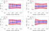 |
Fig. 11. Evolution of concentrations as a function of burnup for relevant fission products for the assembly benchmark. |
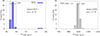 |
Fig. 12. Evolution of the 241Am concentrations from EOL to the cooling time of 7970 days, from the assembly benchmark. Same relative x-scale is used in both histograms. |
As mentioned, 241Am is also a relevant contributor, with about 8% of the total decay heat. Due to the decay of 241Pu, the concentration of 241Am strongly increases after EOL, from 50–100 g/t to 10 times more during the measurement period. Its standard deviation, being large at the EOL (about 20–30% for both models), decreases to about 2% at the measurement time. In addition, the two outliers indicated in green in the figure are becoming closer to the average after EOL, which lowers the standard deviation. As mentioned in Section 4.8, the standard deviation of the 241Am contribution to the total decay heat is also about 2%, corresponding to its concentration spread after EOL.
Finally, 244Cm also contributes to about 10% of the total decay heat. Due to its relatively short half-life (18.1 years), its concentration is decreasing by a factor two to three during the decay heat measurements, but the standard deviation is not changed and stay constant at about 7% for the assembly model (and 4% for the pincell model). The two outliers indicated in green (#13 and #14) strongly increases the standard deviation, and represent higher 244Cm (with 242Pu and 243Am, as they are in the build-up chain of 244Cm) from the first cycle.
A final remark for the minor actinides and their calculated concentrations concerns branching ratios for capture cross sections leading to ground or metastable states. The most relevant example is for the reactions 241Am(n,γ)242mAm and 241Am(n,γ)242gAm (similarly for 243Am). Such branching ratios define the proportions of metastable and ground states and can influence number densities for heavier actinides. Depending on the simulation code, options used during the depletion calculation and the information provided in the nuclear data library, branching ratios can be considered as incident-neutron energy dependent or constant derived from a single energy value or from a (PWR) spectrum average. Such differences may lead to disagreements between actinide concentrations predicted by different codes for 242mAm.
Regarding fission products, four examples are presented in Figure 11 for cases contributing to the total decay heat.
90Sr and 137Cs each contribute to about 30%, when considering their respective decay daughters 90Y and 137mBa. 154Eu and 134Cs contribute to about 1% each, but are among the 11 most important contributors for this specific cooling period. For the most relevant fission products, the spread of calculations is relatively narrow, even considering the outliers highlighted in green. For both the pincell and assembly models, standard deviations for the most relevant fission products are less than 1%.
In the case of 137Cs, all low values are obtained with the same burnup code (cases #37 to #42). The outlier (number #42) uses the JENDL-5 fission yield library, which contains lower cumulative fission yields for 137Cs, from 235U and 239Pu, as presented in reference [26]. In reference [27], the standard deviation obtained for this nuclide during the blind benchmark is close to 1.4%, well in agreement with the values obtained here for the pincell and assembly benchmarks (1.2% at EOL, as indicated in Tab. B.33).
For 134Cs and 154Eu, some outliers can be observed (still having little impact on the decay heat values), especially for case #23.
Regarding the values from the ULC calculations, very similar averages and standard deviations are obtained (see Appendix B), for all the relevant fission products. In general, the standard deviations for the pincell benchmark are smaller than those for the assembly benchmark. The simplicity of the pincell model can partly explain these differences, even if there is not a full overlap between participants for both benchmarks.
4.7. Concentrations during cooling times
The cooling times of interest correspond to the period of calorimetric measurements, from 5823 to 7970 days (or almost 16 to 22 years). Depending on the half-life and decay mode of the nuclides of interest, concentrations can change (as for 241Am, 244Cm, 137Cs or 90Y) and impact the decay heat values (and standard deviations).
A specific example of the impact of the cooling time is 241Am. As previously mentioned, its concentration is strongly changing (increasing), due to the decay of 241Pu. Therefore, the EOL concentration of 241Am is negligible compared to the part coming from 241Pu, and the 241Am spread (standard deviation) at the time of decay heat measurement is similar to the one of 241Pu. This case is presented in Figure 12. One can observe an important reduction in the spread of calculated values after 22 years.
For other cases of relevance for the decay heat, distributions of nuclide concentrations are relatively similar at EOL and measurement times (changes in the spread of the concentration can be observed when a nuclide is decaying into another one, leading to very different concentrations for the considered daughter).
4.8. Decay heat contributors
As mentioned, the decay heat measurements were performed between 5823 and 7970 days of cooling time. For this cooling period, the main contributors were identified in a number of publications (see for instance Refs. [9, 12, 28]). They were requested from each participant, at the measurement times. The contributions from these eleven nuclides (5 actinides 238 − 240Pu, 241Am, 244Cm, and 4 fission products 90Sr, 134, 137Cs, 154Eu and 2 short-lived daughters of relatively long-lived fission products 90Y, 137mBa) are presented in Figure 13 from the calculations of the assembly benchmark. Values of the relative contributions are also presented in Table 9 (and in Appendix B), in the case of the pincell and assembly benchmarks. Additionally, the ULC values are very close to the ones from the direct analysis, and only the ULC set is presented in the Table 9. The sum of these contributions is not 1, but close to 0.99 for both models, indicating the decay heat component of the nuclides not given in this list. These values are in good agreement with the literature values, and the changes for the decay heat measurements at longer cooling time (DH2 to DH6) slightly modify the amplitudes of the contributions. One can note that the standard deviations (1σ) given in the table are relatively small, indicating very good agreement between all individual values.
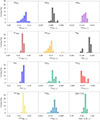 |
Fig. 13. Histograms from participants’ values for the 11 most important decay heat contributors for the cooling time corresponding to the first decay heat measurement DH1 (5823 days). X-scales: contribution to the total decay heat. Bottom right: histogram of the C/E values for the DH1. |
Additionally, small but significant differences can be seen between the pincell and the assembly benchmarks: actinides are contributing more in the case of the pincell (the sum of the actinide contribution is 0.337 for the pincell model, vs. 0.310 for the assembly model). This difference originates in the higher actinide production for the pincell model, due to a different moderator to fissile value H/M. As an example, such a difference represents 46 Watts for actinides and 2 W for fission products, in the case of the first cooling time (5823 days). As shown in the next section, differences of about 40 to 50 W modify the C/E values by 2 to 3%.
Individual nuclide contributions to the decay heat are presented in Figure 13 (along with C/E values), with x-scales kept the same in relative values so that all spreads can be compared. One specific histogram is obtained from all participants’ calculated values. It can be observed that the spread of the DH1 C/E values is very similar to the one of 137mBa, 90Y and 141Am. These three nuclides contribute to about 60% of the total decay heat, and their standard deviations are naturally close to the one for the sum of the DH1 distribution.
As indicated, the main contributors to the six decay heat measurements are limited in number and well identified. Therefore the comparison with decay heat values, within this cooling range, can help to validate only at maximum these 11 nuclides, for both the pincell or assembly benchmarks. In the next section, the values of the calculated decay heat will be compared to the measured ones. For the calculations of the total decay heat, all relevant contributors are considered by the participants, i.e. not only the eleven mentioned nuclides.
4.9. Decay heat C/E values
In this section, the analysis of the calculated decay heat values with respect to the measured ones is presented. As indicated, all relevant decay heat contributors are considered, extending the previous list of 11 nuclides. For convenience, the analysis is separated between the pincell and assembly benchmarks. The main reason is that for the pincell, the calculated decay heat values are generally overestimated, due to its lowed H/M moderation ratio compared to the assembly.
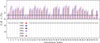 |
Fig. 14. Relative differences between calculated and measured decay heat for the pincell benchmark. Experimental uncertainties are indicated in solid black curves. |
Calculated over Experimental values (C/E) in the case of the pincell benchmark, for the six decay heat measurements (average and 1 standard deviation), obtained from all participants. Only direct (named “quantity All”) and ULC values are presented here, and other values can be found in appendix.
4.9.1. Pincell model
As previously mentioned, the calculated decay heat is expected to be higher than the measured one due to the low moderation ratio for the pincell model. As indicated earlier, this leads to an overproduction of actinides contributing to the decay heat (such as 238Pu, 244Cm). The values of the averages and one standard deviation are presented in Table 10, and histograms are plotted in Figure 1 (left). Individual values for each of the six decay heat values are presented in Figure 14. The x-axis corresponds to the index given in Table 2. Additional statistical values can be found in Tables B.38 and B.39.
The first remark is that for all measurements, the C/E values are higher than 1, and consequently, the average  is also higher than 1, reaching 1.03. The standard deviations are small enough to make all results consistently higher than 1 with a high degree of probability, which is reflected in the tolerance limits given in Appendix B. This is expected for the mentioned reasons, but it is worth observing that all calculations are systematically higher than the measurements (only three sets of calculations are within one experimental standard deviation). Small differences are obtained from the simple average and the ULC approach, indicating that results are independent of the considered codes, libraries, and possible effects from users.
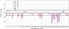 |
Fig. 15. Relative differences between calculated and measured decay heat for the assembly benchmark. Experimental uncertainties are indicated in solid black curves. |
Calculated over Experimental values (C/E) in the case of the assembly benchmark, for the six decay heat measurements (average and 1 standard deviation), obtained from all participants. Only direct (named “quantity All”) and ULC values are presented here, and other values can be found in appendix.
Cases the closest to C/E = 1 (#11, #12, #24, or #51) have a limited overlap in terms of codes and libraries, and originate from different institutes; there is no preferred sets for decay heat calculations given the pincell benchmark, but a tendency to low C/E values is observed for previous JEFF libraries (JEF-2.2, JEFF-3.1.1 and JEFF-3.2), in contrary to JEFF-3.3. With the exception of cases #51 and #52, a common trend can be observed: similar differences between the six measurements are obtained: for a given participant, the highest C/E is obtained for DH4, followed by DH6, DH2, DH5, DH3 and DH1. Such pattern is less pronounced for the results of the assembly model, possibly due to the complexity of the assembly model, leading to more diverse model variations.
On average, 2 to 3% overestimation of the measured decay heat (with a small standard deviation) can be considered adequate, depending on the user’s criteria of acceptance. The systematic overestimation is nevertheless an indication that this benchmark model leads to a bias, which is not present for the assembly model. A possibility to avoid such systematic overestimation is to modify the pincell dimensions to obtain a moderation ratio close to the assembly model.
4.9.2. Assembly model
Similar to the pincell model, results are presented in Table 11, Figure 15 and in Appendix B. Both Figures 10 and 15 have the same y-scale to ease the comparison of results. The main difference with the pincell benchmark is that C/E values are more varying between each participant (or index), and are also lower and higher than 1. The majority of calculations are nevertheless lower than the measurements, leading to an average  close to 0.99. This value indicates a small bias, close to −1%, similar in magnitude to the experimental uncertainties.
The assembly benchmark is more realistic than in the case of the pincell, leading to an average bias closer to zero with a larger standard deviation. In addition, the ULC standard deviation is lower than the one obtained directly from averaging all results together, as indicated in the mentioned tables: from 0.015 to 0.012, while the average C/E values are similar. The use of unique transport and depletion code (line “C” in Tabs. B.38 and B.39) is lowering most the standard deviations, while increasing the average C/E. This can also be observed in Figure 15, where the group of indexes from #37 to #42, leading to low C/E values, are obtained with the same code (see Tab. 2). These six cases (from #37 to #42) underline the effect of nuclear data, as they only differ by the use of the nuclear data library (note that calculation #40, performed with JEFF-3.3, represents the smallest bias from the group).
As this set of indexes also corresponds to a specific institute, results from unique users also lead to low standard deviations and higher C/E.
Calculated over Experimental values (C/E) with standard methods.
From Figure 15, one can see that a small number of calculations have C/E values systematically above 1. Given the number of participants, a similar observation can be made for reference [4], where 3 sets (participants) out of 31 also provide values with C/E > 1 (in this work, numbers are 6 out of 43). The amplitude of the bias is nevertheless smaller for the present benchmark (−1.1% compared to −2.0% in Ref. [4]).
4.10. Standard methods
Standard methods are often used to calculate assembly decay heat in a simplified manner, based on a set of predefined functions and parameters, possibly complemented with simplified depletion chains. The most common decay heat standards are the DIN 25463-1:2014 [29] (called DIN 2014), the ANSI/ANS-5.1:2014 [30] (called ANS 2014), and more recently the US NRC Regulatory guide 3.54, revision 2 [31] (called RG-3.54 2018), the US NRC Regulatory guide 3.54, revision 3 [32] (called RG-3.54 2022) and the ISO 10645:2022 [33] (called ISO 2022).
The results of standard methods are provided here as an indication of what they provide for the 0E2 assembly. They are not based on the benchmark descriptions. These methods do not require a geometry description, but simplified information such as cooling time, initial fuel composition, mass and burnup. They are often conservative in the sense that they provide decay heat values higher than those obtained from a detailed calculation, except for the DIN standard, which is expected to be closer to best-estimate values. Each of these standards has its own range of applicability (limits in final burnup, initial enrichment, cooling range), and for the considered assembly 0E2, all the mentioned standards can be applied. Table 12 presents the C/E values obtained with the four standards, using the implementation from the Studsvik code called stdsnf (as applied in Ref. [1]), except for the standard RG-3.54 2022, for which the decay heat estimator widget as implemented in a beta version of SCALE 7.0 is used [34].
As observed, apart from the DIN 2014 standard, other ones provide C/E values greater than 1, and also generally greater than the values obtained with transport and depletion codes. Standard values for the current benchmark are similar to the ones from reference [9]. If one is interested by conservative values of the decay heat, or by obtaining values without setting up a geometrical model, these standards offer a convenient solution. They are naturally limited to specific fuel enrichment, content, burnup and cooling time, which can justify the use of transport codes. Additionally, if one needs less conservative values, standards are generally not recommended (it was shown in Ref. [9] that the DIN standard might not be systematically conservative).
4.11. Detailed operational history
Additional information can potentially influence the estimation of the calculated decay heat. For the assembly 0E2, SKB has access to a more detailed operational history than the one provided to the other participants in this study. To investigate the effect of this detailed history, a calculation of the decay heat was made with an operational history consisting of approximately 25 steps for each cycle. Each step was depleted with an individual value on moderator-and fuel-temperature, boron concentration and power, for each of the 24 axial nodes. To make a comparison, a calculation was also made with the code SNF-1.8 and the nuclear data library ENDF/B-VII.1. with the same data as provided to the other participants. The results can be seen in Table 13. The C/E − 1 average for the detailed operational history is 0.5 percent higher than the 2D average data. The results for the 2D average data are very close to the average result of the other participants in this study. To further investigate how much of this difference is due to 2D/3D effect and how much is depending on the detailed history a comparison was made with Polaris using the same input, only changing 2D to 3D, see results in Table 14.
Comparisons of the calculated over Experimental values (C/E − 1) with detailed operational history, and without (simplified 2D calculation). Calculations were performed with SNF-1.8: coupled to a 3D core simulator for the left column, and using information as provided in this benchmark for the right column.
Comparisons of the calculated over Experimental values (C/E − 1) with detailed operational history (3D), and without (simplified 2D calculation). Calculations are performed with Polaris (see text for details).
One can conclude that most of the difference between the cases in Table 13 are due to the 2D/3D effect. Detailed operational history for an assembly with long cooling times as 0E2 only effects the results with a few parts of a percent.
Summary table of the calculated uncertainties (Δ corresponds to 1σ) for both benchmarks. For the decay heat, the C/E − 1 ±1σ over the six measurements is given. RR means fission reaction rates. For all quantities except the decay heat, values are given at EOL. If not specified, uncertainties concern nuclide concentrations. Data comes from the ULC analysis.
5. Main outcomes
General conclusions and outcomes from the present study are succinctly summarized in the following. Details can be found in the previous sections and in Appendix B. Participants, codes and libraries can be found in Table 2, and individual details are provided in Appendix C.
For the pincell benchmark:
-
38 different calculations were performed for this benchmark (see Tab. 3).
-
It has the advantage to require a limited amount of computer power, but it was observed that the moderation H/M ratio for the pincell benchmark is too low compared to a realistic assembly case, leading to a larger production of actinides heavier than uranium.
-
The decay heat is overestimated by all participants with an average bias of ( + 2.6 ± 0.9)% (being C/E − 1 ± 1σ) (see Tab. 10 and Fig. 14).
For the assembly benchmark:
-
43 different calculations were performed for the 2D assembly benchmark. It is more realistic than the pincell benchmark, but requires more computational power, especially for Monte Carlo transport simulations.
-
Results of all participants indicate a good agreement with the measurements, corresponding to an average bias of ( − 1.1 ± 1.2)% (being C/E − 1 ± 1σ). Given the experimental uncertainty of 1.2 to 1.3%, the agreement between calculated and measured values is judged to be satisfactory (see Tab. 11 and Fig. 15).
Additionally, general remarks about the calculations performed in this work are as follows.
-
A majority of participants used a Monte Carlo neutron transport code (SERPENT) and the ENDF/B-VII.1 nuclear data library. Simple analysis of results are therefore biased towards this code and library. It is proposed to use statistical quantities (among which averages and standard deviations) obtained from unique sets of codes, libraries and participants. These values are recommended (named “ULC” and presented in bold in various tables).
-
Given the long cooling time of the six considered measurements for the PWR UO2 assembly 0E2, a limited number of nuclides contributes to the decay heat, mainly 137mBa/137Cs, 90Y/90Sr, 244Cm, 238Pu and 241Am (see Tab. 9). These nuclides are in fact the main contributors to a vast majority of calorimetric decay heat measurements performed at long cooling times, as noticed in various publications.
-
The present study provides averages and standard deviations for other nuclides of interest to decay heat and criticality-safety calculations, along with quantities such as k∞ and reaction rates. Uncertainties (as the standard deviations from the values of participants) for these values are given in the summary provided in Table 15 (at EOL, except for the decay heat, given as an average at the measurement times). These standard deviations (1σ) can be useful when evaluating uncertainties to be taken into account for criticality-safety calculations and burnup credit.
-
Two additional sets of calculations, performed outside the benchmark exercise (1) confirmed that the standard methods are generally conservative, except the DIN standard which is closer to the benchmark values, and (2) indicated that additional consideration of the assembly detailed operating and nodal data modifies the calculated decay heat by a few tenths of a percent.
6. Conclusion
Two decay heat benchmarks were created in the context of the OECD NEA WPNCS subgroup 16, based on the PWR UO2 Westinghouse 17 × 17 assembly, named 0E2, from the Ringhals-3 reactor, in Sweden. One simplified benchmark consists of a pincell model, and the other benchmark represents an assembly, both being two-dimension models. The 0E2 assembly had an initial 235U enrichment of 3.1%, was irradiated for four cycles, up to 41.6 MWd/kg. Six calorimetric decay heat measurements were realized for this assembly, between 16 and 22 years of cooling time.
A total of 38 pincell and 43 assembly calculations were performed by 21 participants, providing the following quantities: decay heat at the time of measurements, k∞, reaction rates, nuclide concentrations and decay heat contributors. Such benchmark calculations were performed while the measurement values were already available, but calculation results have been submitted by each participant without knowing the results of others.
A large variety of codes, libraries and modeling approach has been used, covering deterministic and Monte Carlo neutron transport (and depletion) codes, and modern nuclear data libraries as well as early ones. The Monte Carlo code Serpent was used a large number of times, and similarly, the nuclear data library ENDF/B-VII.1 was also over-represented. In order to compensate for this effect, averages and standard deviations based on a single code/library/participant representation are also provided with the values directly obtained from the unprocessed set of results.
It was found that the decay heat values are overestimated by all participants in the case of the pincell benchmark, with C/E − 1 ± 1σ of (+2.6 ± 0.9)%. This is expected as the moderation ratio is under-estimated in the pincell benchmark, compared to a realistic fuel assembly. For the assembly model, the average bias is smaller, with ( − 1.1 ± 1.2)%.
In addition, uncertainties are provided for other not-measured quantities, such as k∞ at the beginning of irradiation and for each cycle, the nuclide concentrations at the end of irradiation, and fission reaction rates. The uncertainties correspond to the spread (1σ) of the results compared to the average calculated quantities. These quantities are also of interest for criticality-safety calculations.
Funding
This research did not receive any specific funding.
Conflicts of interest
The authors declare that they have no competing interests to report.
Data availability statement
This article has no associated data generated or analyzed.
Author contribution statement
All authors equally contributed to the generation of data, calculations, analysis and writing.
References
- D. Rochman, A. Algora, F. Àlvarez-Velarde, A. Bardelay, Ø. Bremnes, O. Cabellos, D. Cano-Ott, L. Capponi, C. Carmouze, S. Caruso, A. Cummings, R. Dagan, M. Fallot, L. Fiorito, L. Giot, K. Govers, S. Häkkinen, V. Hannstein, A. Hoefer, T.D. Huynh, R. Ichou, G. Ilas, P. Juutilainen, L. Koszuk, M. Kromar, S. Lahaye, J. Lam, F. Laugier, A. Launay, V. Léger, D. Lecarpentier, J. Leppanen, F. Malouch, J.F. Martin, D. McGinnes, R.W. Mills, F. Minato, Y. Nauchi, P. Ortego, P. Petkov, P. Romojaro, S. Sato, M. Seidl, A. Shama, T. Simeonov, A. Sjöland, V. Solans, F. Sommer, S. Tittelbach, A. Tsilanizara, E. Vlassopoulos, V. Vallet, A. Vasiliev, T. Watanabe, G. Žerovnik, An introduction to spent nuclear fuel decay heat for light water reactors: a review from the NEA WPNCS, EPJ Nucl. Sci. Technol. 10, 9 (2024), https://doi.org/10.1051/epjn/2024010 [Google Scholar]
- H. Akkurt, R. Hall, F. Johansson, A. Mehic, J. Kierkegaard, H. Liljenfeldt, Spent fuel decay heat measurements at clab: description of decay heat measurements from 2003–2021 under EPRI-SKB collaboration, Tech. Rep. 000000003002026549, Electric Power Research Institute, EPRI, USA, October 2024, https://www.epri.com/research/programs/061149/results/3002026549 [Google Scholar]
- F. Sturek, L. Agrenius, Measurements of decay heat in spent nuclear fuel at the Swedish interim storage facility, Clab, Tech. Rep. R-05-62, Svensk Kärnbränslehantering AB (SKB), Sweden, December 2006, https://www.skb.se/publikation/1472024/R-05-62.pdf [Google Scholar]
- P. Jansson, M. Bengtsson, U. Bäckström, F. Àlvarez-Velarde, D. Calic, S. Caruso, R. Dagan, L. Fiorito, L. Giot, K. Govers, A.H. Solis, V. Hannstein, G. Ilas, M. Kromar, J. Leppänen, M. Mosconi, P. Ortego, R. Plukiene, A. Plukis, A. Ranta-aho, D. Rochman, L. Ros, S. Sato, P. Schillebeeckx, A. Shama, T. Simeonov, A. Stankovskiy, H. Trellue, S. Vaccaro, V. Vallet, M. Verwerft, G. Žerovnik, A. Sjöland, Blind benchmark exercise for spent nuclear fuel decay heat, Nucl. Sci. Eng. 196, 1125 (2022), https://doi.org/10.1080/00295639.2022.2053489 [CrossRef] [Google Scholar]
- I.C. Gauld, G. Ilas, B.D. Murphy, C.F. Weber, Validation of SCALE 5 decay heat predictions for LWR Spent Nuclear Fuel, Tech. Rep. ORNL/TM-2008/015 and NUREG/CR-6972, Oak Ridge National Laboratory, USA, February 2010, https://www.nrc.gov/docs/ML1009/ML100900229.pdf [Google Scholar]
- O.W. Hermann, C.V. Parks, J.P. Renier, Technical support for a proposed decay heat guide using Sas2H/Origen-S data, Tech. Rep. NREG/CR-5625, ORNL-6698, Oak Ridge National Laboratory, September 1994, https://www.osti.gov/servlets/purl/43752 [Google Scholar]
- G. Ilas, I.C. Gauld, H. Liljenfeldt, Validation of origen for LWR used fuel decay heat analysis with scale, Nucl. Eng. Des. 273, 58 (2014), https://doi.org/10.1016/j.nucengdes.2014.02.026 [Google Scholar]
- D. Rochman, Decay heat computational comparison exercise: definition for a PWR UO2 assembly and pincell; specifications for the exercise of WPNCS SG16, Tech. Rep., Nuclear Energy Agency, NEA/NSC/WPNCS/WD(2024)1/REV1, 2024 [Google Scholar]
- D. Rochman, J. Taforeau, T. Simeonov, A. Shama, Comparison of calculated and measured spent nuclear fuel decay heat with CASMO5, SNF and standard methods, Nucl. Eng. Des. 410, 112392 (2023), https://doi.org/10.1016/j.nucengdes.2023.112392 [Google Scholar]
- A. Shama, D. Rochman, S. Caruso, A. Pautz, Validation of spent nuclear fuel decay heat calculations using Polaris, ORIGEN and CASMO5, Ann. Nucl. Energy 165, 108758 (2022), https://doi.org/10.1016/j.anucene.2021.108758 [CrossRef] [Google Scholar]
- J. Jang, B. Ebiwonjumi, W. Kim, J. Park, J. Choe, D. Lee, Validation of spent nuclear fuel decay heat calculation by a two-step method, Nucl. Eng. Technol. 53, 44 (2021), https://doi.org/10.1016/j.net.2020.06.028 [Google Scholar]
- G. Ilas, I.C. Gauld, SCALE analysis of CLAB decay heat measurements for LWR spent fuel assemblies, Ann. Nucl. Energy 35, 37 (2008), https://doi.org/10.1016/j.anucene.2007.05.017 [CrossRef] [Google Scholar]
- P.K. Romano, C.J. Josey, A.E. Johnson, J. Liang, Depletion capabilities in the OpenMC Monte Carlo particle transport code, Ann. Nucl. Energy 152, 107989 (2021), https://doi.org/10.1016/j.anucene.2020.107989 [CrossRef] [Google Scholar]
- E. Brun, A. Zoia, J.C. Trama, S. Lahaye, Y. Nagaya, Inter-code comparison of TRIPOLA and MVP on the MCNP criticality validation suite, in Proceedings of the ICNC-2015, International Conference on Nuclear Criticality Safety Conference (Charlotte, NC, September 13–17, 2015), p. 351, https://cea.hal.science/cea-02489517/document [Google Scholar]
- H.J. Park, H. Kang, H.C. Lee, J.Y. Cho, Comparison of ENDF/B-VIII.0 and ENDF/B-VII.1 in criticality, depletion benchmark, and uncertainty analyses by McCARD, Ann. Nucl. Energy 131, 443 (2019), https://doi.org/10.1016/j.anucene.2019.04.012 [Google Scholar]
- F. Michel-Sendis, I. Gauld, J.S. Martinez, C. Alejano, M. Bossant, D. Boulanger, O. Cabellos, V. Chrapciak, J. Conde, I. Fast, M. Gren, K. Govers, M. Gysemans, V. Hannstein, F. Havluj, M. Hennebach, G. Hordosy, G. Ilas, R. Kilger, R. Mills, D. Mountford, P. Ortego, G. Radulescu, M. Rahimi, A. Ranta-Aho, K. Rantamäki, B. Ruprecht, N. Soppera, M. Stuke, K. Suyama, S. Tittelbach, C. Tore, S.V. Winckel, A. Vasiliev, T. Watanabe, T. Yamamoto, T. Yamamoto, SFCOMPO-2.0: An OECD NEA database of spent nuclear fuel isotopic assays, reactor design specifications, and operating data, Ann. Nucl. Energy 110, 779 (2017), https://doi.org/10.1016/j.anucene.2017.07.022 [CrossRef] [Google Scholar]
- C. Carmouze, R. Ichou, G. Ilas, F. Alvarez-Velarde, M. Chernykh, R. García-Baonza, L. Giot, K. Govers, F. Grimaldi, V. Hannstein, A. Hoefer, P. Juutilainen, J. Lams, P. Martinez-Moreno, D. Mennerdahl, U. Mertyurek, Y. Molla, S. Richards, D. Rochman, P. Romojaro, D.S. Grachtrup, A. Shama, N. Slosse, P. Smith, F. Sommer, M.S. Skrodzka, S. Tittelbach, T.W.G. Žerovnik, Overview of spent nuclear fuel inventory results for the ARIANE GU3 sample, in Proceedings of the ICNC-2023, International Conference on Nuclear Criticality Safety Conference (Sendai, Japan, October 1–6, 2023), https://www.osti.gov/biblio/2333758 [Google Scholar]
- J.D. Bess, T. Ivanova, I. Hill, J.-F. Martin, J.B. Briggs, L. Scott, M. DeHart, C. Percher, B.J. Marshall, P. Blaise, Intrinsic value of the international benchmark projects, ICSBEP and IRPhEP, for advanced reactor development, Front. Energy Res. 11 (2023), https://doi.org/10.3389/fenrg.2023.1085788 [Google Scholar]
- M. Frankl, A. Vasiliev, D. Rochman, H. Ferroukhi, M. Wittel, S. Pudollek, Refinement of the loading curve determination methodology and modeling for Swiss PWR spent fuel final disposal canisters, in Proceedings of the ICNC-2023, International Conference on Nuclear Criticality Safety Conference (Sendai, Japan, October 1–6, 2023), https://www.researchgate.net/publication/377207109_REFINEMENT_OF_THE_LOADING_CURVE_DETERMINATION_METHODOLOGY_AND_MODELING_FOR_SWISS_PWR_SPENT_FUEL_FINAL_DISPOSAL_CANISTERS [Google Scholar]
- M. Frankl, M. Hursin, D. Rochman, A. Vasiliev, H. Ferroukhi, Nuclear data uncertainty quantification in criticality safety evaluations for spent nuclear fuel geological disposal, Appl. Sci. 11, 6499 (2021), https://doi.org/10.3390/app11146499 [CrossRef] [Google Scholar]
- D. Rochman, O. Leray, G. Perret, A. Vasiliev, H. Ferroukhi, A. Koning, Re-evaluation of the thermal neutron capture cross section of 147Nd, Ann. Nucl. Energy 94, 612 (2016), https://doi.org/10.1016/j.anucene.2016.03.024 [Google Scholar]
- D. Rochman, A. Vasiliev, H. Ferroukhi, M. Hursin, R. Ichou, J. Taforeau, T. Simeonov, Analysis for the ARIANE GU3 sample: nuclide inventory and decay heat, EPJ Nucl. Sci. Technol. 7, 14 (2021), https://doi.org/10.1051/epjn/2021013 [CrossRef] [EDP Sciences] [Google Scholar]
- D. Rochman, A. Vasiliev, H. Ferroukhi, M. Hursin, Analysis for the ARIANE BM1 and BM3 samples: nuclide inventory and decay heat, EPJ Nucl. Sci. Technol. 7, 18 (2021), https://doi.org/10.1051/epjn/2021017 [Google Scholar]
- D. Rochman, A. Vasiliev, H. Ferroukhi, M. Seidl, J. Basualdo, Improvement of PIE analysis with a full core simulation: the U1 case, Ann. Nucl. Energy 148, 107706 (2020), https://doi.org/10.1016/j.anucene.2020.107706 [CrossRef] [Google Scholar]
- G. Žerovnik, P. Schillebeeckx, K. Govers, A. Borella, D. Calic, L. Fiorito, B. Kos, A. Stankovskiy, G. van der Eynde, M. Verwerf, Observables of interest for the characterization of Spent Nuclear Fuel, Tech. Rep. EUR 29301 EN, Publications Office of the European Union, Luxembourg, 2018, https://publications.jrc.ec.europa.eu/repository/bitstream/JRC112361/report_eur_29301en.pdf [Google Scholar]
- P. Schillebeeckx, M. Verwerft, P. Romojaro, G. Žerovnik, N. Messaoudi, G. Alaerts, L. Fiorito, K. Govers, J. Paepen, Y. Parthoens, B. Pedersen, A. Stankovskiy, G. Van den Eynde, R. Wynants, An absolute measurement of the neutron production rate of a spent nuclear fuel sample used for depletion code validation, Front. Energy Res. 11, 1162367 (2023), https://doi.org/10.3389/fenrg.2023.1162367 [CrossRef] [Google Scholar]
- P. Jansson, M. Bengtsson, U. Bäckström, K. Svensson, M. Lycksell, A. Sjöland, Data from calorimetric decay heat measurements of five used PWR 17x17 nuclear fuel assemblies, Data Brief 28, 104917 (2020), https://doi.org/10.1016/j.dib.2019.104917 [CrossRef] [Google Scholar]
- H. Akkurt, H. Liljenfeldt, G. Ilas, S. Baker, Phenomena Identification and Ranking Table (PIRT) for decay heat, Tech. Rep. 3002018440, Electric Power Research Institute, EPRI, USA, July 2020 [Google Scholar]
- DIN Standards Committee Materials Testing, Calculation of the decay power in nuclear fuels of light water reactors – Part 1: uranium oxide nuclear fuel for pressurized water reactors, English translation of DIN 25463-1:2014-02, Tech. Rep. DIN 25463-1:2014-02, DIN Standards Committee Materials Testing, Germany, February 2014 [Google Scholar]
- American Nuclear Society Standards Committee Working Group ANS-5.1, Decay heat power in light water reactors, Tech. Rep. ANSI/ANS-5.1-2014, American Nuclear Society, November 2014 [Google Scholar]
- A. Sotomayor-Rivera, Spent fuel heat generation in an independent spent fuel storage installation, Tech. Rep. US NRC Regulatory Guide 3.54, Rev.2, U.S. Nuclear Regulatory Commission, USA, 2018 [Google Scholar]
- A. Sotomayor-Rivera, Spent fuel heat generation in an independent spent fuel storage installation, Tech. Rep. US NRC Regulatory Guide 3.54, Rev.3, U.S. Nuclear Regulatory Commission, USA, 2022, https://www.nrc.gov/docs/ML2206/ML22067A014.pdf [Google Scholar]
- Technical Committee ISO/TC 85, Nuclear energy, Sub-Committee SC 6, Power reactor technology, Nuclear energy – Light water reactors – Calculation of the decay heat power in nuclear fuels, Tech. Rep., ISO International Standard, April 2022 [Google Scholar]
- S. Skutnik, Emerging visualization and utility capabilities for FULCRU, in SCALE Users’ Group Workshop (June 5–7, Oak Ridge National Laboratory, Oak Ridge, USA, 2024), https://www.ornl.gov/file/2024-sug-workshop-emerging-visualization-and-utility-capabilities-fulcrum/display [Google Scholar]
- A. Stankovskiy, G. Van den Eynde, Advanced method for calculations of core burn-up, activation of structural materials, and spallation products accumulation in accelerator-driven systems, Sci. Technol. Nucl. Install. 2012, 545103 (2012), https://doi.org/10.1155/2012/545103 [Google Scholar]
- R. Ferrer, J. Rhodes, Generation and initial validation of a new CASMO5 ENDF/B-VIII.0 nuclear data library, in Proceedings of the PHYSOR 2020 (March 29–April 2, Cambridge, UK, 2020) [Google Scholar]
- J. Rhodes, K. Smith, D. Lee, CASMO-5 Development and Applications, in Proceedings of the PHYSOR 2006 (September 10–14, Vancouver, BC, Canada, 2006), p. B144, https://www.studsvik.com/SharepointFiles/CASMO-5%20Development%20and%20Applications.pdf [Google Scholar]
- A. Persic, A. Trkov, The energy released by neutron capture in thermal reactors, 1999, https://inis.iaea.org/records/ceygs-34k05 [Google Scholar]
- L. San-Felice, R. Eschbach, P. Bourdot, Experimental validation of the DARWIN2.3 package for fuel cycle applications, Nucl. Technol. 184, 217 (2013), https://doi.org/10.13182/NT12-121 [Google Scholar]
- A. Santamarina, D. Bernard, P. Blaise, P. Leconte, R. Le Tellier, C. Vaglio-Gaudard, J.-F. Vidal, APOLLO2.8: a validated code package for PWR neutronics calculations, in 4th Topical Meeting on Advances in Nuclear Fuel Management 2009, ANFM IV (American Nuclear Society, Vol. 2, 2009) [Google Scholar]
- A. Tsilanizara, T. Huynh, New feature of DARWIN/PEPIN2 inventory code: propagation of nuclear data uncertainties to decay heat and nuclide density, Ann. Nucl. Energy 164, 108579 (2021), https://doi.org/10.1016/j.anucene.2021.108579 [CrossRef] [Google Scholar]
- A. Santamarina, D. Bernard, P. Blaise, M. Coste, A. Courcelle, T. Huynh, C. Jouanne, P. Leconte, O. Litaize, S. Mengelle, G. Nogue, J.-M. Ruggiéri, O. Sérot, J. Tommasi, C. Vaglio, J.-F. Vidal, The JEFF-3.1.1 nuclear data library: JEFF report 22: validation results from JEF-2.2 to JEFF-3.1.1, Tech. Rep., Nuclear Energy Agency of the OECD (NEA), 2009, https://www.oecd-nea.org/upload/docs/application/pdf/2019-12/nea6807-jeff22.pdf [Google Scholar]
- F. Àlvarez Velarde, E. Gonzàlez-Romero, I.M. Rodrìguez, Validation of the burn-up code EVOLCODE 2.0 with PWR experimental data and with a Sensitivity/Uncertainty analysis, Ann. Nucl. Energy 73, 175 (2014), https://doi.org/10.1016/j.anucene.2014.06.049 [CrossRef] [Google Scholar]
- T. Goorley, M. James, T. Booth, F. Brown, J. Bull, L. Cox, J. Durkee, J. Elson, M. Fensin, R. Forster, J. Hendricks, H. Hughes, R. Johns, B. Kiedrowski, R. Martz, S. Mashnik, G. McKinney, D. Pelowitz, R. Prael, J. Sweezy, L. Waters, T. Wilcox, T. Zukaitis, Features of MCNP6, Ann. Nucl. Energy 87, 772 (2016), https://doi.org/10.1016/j.anucene.2015.02.020 [CrossRef] [Google Scholar]
- J. Sanz, O. Cabellos, N. García-Herranz, ACAB Inventory code for nuclear applications: user’s manual V. 2008, NEA-1839 6, 475 (2008) [Google Scholar]
- C. Wemple, H.-N. Gheorghiu, R. Stamm’ler, E. Villarino, Recent advances in the HELIOS-2 lattice physics code, in Proceedings of the Intl. Conf. on the Physics of Reactors (PHYSOR) (Sept. 14–19, Interlaken, Switzerland, 2008) [Google Scholar]
- W.A. Wieselquist, E.R.A. Lefebvre, SCALE 6.3.1 user manual, Tech. Rep., Oak Ridge National Laboratory, ORNL/TM-SCALE-6.3.1, 2023, https://doi.org/10.2172/1959594 [Google Scholar]
- T. Simeonov, C. Wemple, Advances in Studsvik’s system for spent fuel analysis, EPJ Web Conf. 247, 02021 (2021), https://doi.org/10.1051/epjconf/202124702021 [CrossRef] [EDP Sciences] [Google Scholar]
- W. Haeck, B. Decheneaux, VESTA user’s manual – version 2.2.0, Tech. Rep. PSN-EXP/SNC/2017-00251, IRSN, France, 2017 [Google Scholar]
- B. Cochet, A. Jinaphanh, L. Heulers, O. Jacquet, Capabilities overview of the MORET 5 Monte Carlo code, Ann. Nucl. Energy 82, 74 (2015), https://doi.org/10.1016/j.anucene.2014.08.022 [Google Scholar]
Organisation for Economic Co-operation and Development.
In the following, the unit will be MWd/kg, corresponding to the notation sometimes found in publications of MWd/kgU or MWd/kgHM; the term kg refers to the initial amount of uranium in the fuel.
In the following the word “rate” will not be repeated.
The unit g/tHM refers to grams per ton of initial heavy metals; for the assembly 0E2, the heavy metals consist only in uranium nuclides.
The notation BOC is not added in this section as there is no ambiguity on the considered quantities.
LCT stands for LEU-COMP-THERM following the ICSBEP definition [18].
Cite this article as: Dimitri A. Rochman, Francisco Alvarez-Velarde, Kelsey Amundson, John Bess, Sebastien Bonthoux, Oscar Cabellos, Coralie Carmouze, Shahab Dabiran-Zohoory, Ron Dagan, Luca Fiorito, Juan García, Lydie Giot, Fernando Gomez Salcedo, Volker Hannstein, Silja Häkkinen, Mathieu Hursin, Raphaelle Ichou, Fredrik Johansson, P. Juutilainen, Marjan Kromar, Sébastien Lahaye, Agnes Launay, Vincent Léger, R.W. Mills, Ugur Mertyurek, Pedro Ortego, Sofia Portolan, Miiko Pöyhönen, Germina Procop, Pablo Romojaro, Benjamin Ruprecht, Bishal Torrente, Sven Tittelbach, S. Sato, A. Shama, T. Simeonov, Virginie Solans, V. Vallet, Alexander Vasiliev, Gasper Žerovnik. The 0E2 benchmarks for PWR UO2 decay heat: an analysis from the NEA WPNCS, EPJ Nuclear Sci. Technol. 12, 20 (2026). https://doi.org/10.1051/epjn/2026011
Appendix
Additional benchmark descriptions
In the following, a number of additional tables are provided, allowing a complete description of the pincell and assembly models. The information provided corresponds to the one used during the SG16 exercise. Specific notes, detailing specific aspects of the selected data are also given (see notes 1 to 6).
General information for assembly 0E2 – part 1.
Note 1. The original temperatures for the coolant and pellets at full power are assumed to be 600 and 900 K, respectively. The original values from reference [3] (page 226/253) are 576 and 850 K. These new benchmark values are assumed in order to ease the nuclear data processing at default temperatures available in most of the processed libraries.
Note 2. For the initial concentration of 234U, no information is given in reference [3]. A correlation with the 235U concentration is then assumed, being 0.89% [6], leading to an initial 234U concentration of 0.276%. The initial concentration of 238U provided in reference [3] is then reduced by the same amount. Regarding the 236U initial concentration, it is assumed to be zero. Note that this concentration does not correspond to typical Swedish fuel.
Note 3. The effective fuel density is calculated from the active length and the initial heavy mass weight provided in reference [3]. The value of pellet density (10.45 g/cm3) and pellet density including chamfer, dishing, etc. (10.35 g/cm3) provided in reference [3] (page 227/253) is not used. Instead, the following effective fuel density d is derived:
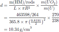 (A.1)
(A.1)
This value is very close to the one provided in reference [3], being 10.35 g/cm3.
Note 4. The value of the reactor power is given, as in reference [3], but shall not be used in the benchmark. Instead, participants are required to use the assembly burnup values, as given in Table A.3.
Note 5. These quantities were not provided in the references [3] and [7] and correspond to ad-hoc assumptions.
Note 6. Mass ratio of boron, as part of the boric acid added to clean water, to mass of borated water.
General information for assembly 0E2 – part 2 (cold dimensions).
General information for assembly 0E2 – part 3.
Description of the pincell model.
Appendix
Statistical quantities
Calculated k∞ values for the pincell and assembly models. Values with a ± sign are average ±σ (σ are given in pcm), whereas values within solid brackets ([ ]) are 95%/95% tolerance limits. In bold are indicated the reference values.
Calculated values for the pincell and assembly models for the 234U concentrations. Values with a ± sign are average ±σ, whereas values within solid brackets ([ ]) are 95%/95% tolerance limits. In bold are indicated the reference values.
Calculated values for the pincell and assembly models for the 234U concentrations (during irradiation and cooling). Values with a ± sign are average ±σ, whereas values within solid brackets ([ ]) are 95%/95% tolerance limits. In bold are indicated the reference values.
Calculated values for the pincell and assembly models for the 235U concentrations. Values with a ± sign are average ±σ, whereas values within solid brackets ([ ]) are 95%/95% tolerance limits. In bold are indicated the reference values.
Calculated values for the pincell and assembly models for the 235U concentrations (during irradiation and cooling). Values with a ± sign are average ±σ, whereas values within solid brackets ([ ]) are 95%/95% tolerance limits. In bold are indicated the reference values.
Calculated values for the pincell and assembly models for the 236U concentrations. Values with a ± sign are average ±σ, whereas values within solid brackets ([ ]) are 95%/95% tolerance limits. In bold are indicated the reference values.
Calculated values for the pincell and assembly models for the 236U concentrations (during irradiation and cooling). Values with a ± sign are average ±σ, whereas values within solid brackets ([ ]) are 95%/95% tolerance limits. In bold are indicated the reference values.
Calculated values for the pincell and assembly models for the 238U concentrations. Values with a ± sign are average ±σ, whereas values within solid brackets ([ ]) are 95%/95% tolerance limits. In bold are indicated the reference values.
Calculated values for the pincell and assembly models for the 238U concentrations (during irradiation and cooling). Values with a ± sign are average ±σ, whereas values within solid brackets ([ ]) are 95%/95% tolerance limits. In bold are indicated the reference values.
Calculated values for the pincell and assembly models for the 235U fission reaction rates (RR), given in %. Values with a ± sign are average ±σ, whereas values within solid brackets ([ ]) are 95%/95% tolerance limits. In bold are indicated the reference values.
Calculated values for the pincell and assembly models for the 238U fission reaction rates (RR), given in %. Values with a ± sign are average ±σ, whereas values within solid brackets ([ ]) are 95%/95% tolerance limits. In bold are indicated the reference values.
Calculated values for the pincell and assembly models for the 239Pu fission reaction rates (RR), given in %. Values with a ± sign are average ±σ, whereas values within solid brackets ([ ]) are 95%/95% tolerance limits. In bold are indicated the reference values.
Calculated values for the pincell and assembly models for the 241Pu fission reaction rates (RR), given in %. Values with a ± sign are average ±σ, whereas values within solid brackets ([ ]) are 95%/95% tolerance limits. In bold are indicated the reference values.
Calculated values for the pincell and assembly models for the 238Pu concentrations during irradiation. Values with a ± sign are average ±σ, whereas values within solid brackets ([ ]) are 95%/95% tolerance limits. In bold are indicated the reference values.
Calculated values for the pincell and assembly models for the 238Pu concentrations during cooling and contribution to decay heat at 5823 days (last column, named “Contrib."). Values with a ± sign are average ±σ, whereas values within solid brackets ([ ]) are 95%/95% tolerance limits. In bold are indicated the reference values.
Calculated values for the pincell and assembly models for the 239Pu concentrations during irradiation. Values with a ± sign are average ±σ, whereas values within solid brackets ([ ]) are 95%/95% tolerance limits. In bold are indicated the reference values.
Calculated values for the pincell and assembly models for the 239Pu concentrations during cooling and contribution to decay heat at 5823 days (last column, named “Contrib."). Values with a ± sign are average ±σ, whereas values within solid brackets ([ ]) are 95%/95% tolerance limits. In bold are indicated the reference values.
Calculated values for the pincell and assembly models for the 240Pu concentrations during irradiation. Values with a ± sign are average ±σ, whereas values within solid brackets ([ ]) are 95%/95% tolerance limits. In bold are indicated the reference values.
Calculated values for the pincell and assembly models for the 240Pu concentrations during cooling and contribution to decay heat at 5823 days (last column, named “Contrib."). Values with a ± sign are average ±σ, whereas values within solid brackets ([ ]) are 95%/95% tolerance limits. In bold are indicated the reference values.
Calculated values for the pincell and assembly models for the 241Pu concentrations during irradiation. Values with a ± sign are average ±σ, whereas values within solid brackets ([ ]) are 95%/95% tolerance limits. In bold are indicated the reference values.
Calculated values for the pincell and assembly models for the 241Pu concentrations during cooling. Values with a ± sign are average ±σ, whereas values within solid brackets ([ ]) are 95%/95% tolerance limits. In bold are indicated the reference values.
Calculated values for the pincell and assembly models for the 242Pu concentrations during irradiation. Values with a ± sign are average ±σ, whereas values within solid brackets ([ ]) are 95%/95% tolerance limits. In bold are indicated the reference values.
Calculated values for the pincell and assembly models for the 242Pu concentrations during cooling. Values with a ± sign are average ±σ, whereas values within solid brackets ([ ]) are 95%/95% tolerance limits. In bold are indicated the reference values.
Calculated values for the pincell and assembly models for the 241Am concentrations during irradiation. Values with a ± sign are average ±σ, whereas values within solid brackets ([ ]) are 95%/95% tolerance limits. In bold are indicated the reference values.
Calculated values for the pincell and assembly models for the 241Am concentrations during cooling and contribution to decay heat at 5823 days (last column, named “Contrib."). Values with a ± sign are average ±σ, whereas values within solid brackets ([ ]) are 95%/95% tolerance limits. In bold are indicated the reference values.
Calculated values for the pincell and assembly models for the 244Cm concentrations during irradiation. Values with a ± sign are average ±σ, whereas values within solid brackets ([ ]) are 95%/95% tolerance limits. In bold are indicated the reference values.
Calculated values for the pincell and assembly models for the 244Cm concentrations during cooling and contribution to decay heat at 5823 days (last column, named “Contrib."). Values with a ± sign are average ±σ, whereas values within solid brackets ([ ]) are 95%/95% tolerance limits. In bold are indicated the reference values.
Calculated values for the pincell and assembly models for the 90Sr concentrations during irradiation. Values with a ± sign are average ±σ, whereas values within solid brackets ([ ]) are 95%/95% tolerance limits. In bold are indicated the reference values.
Calculated values for the pincell and assembly models for the 90Sr concentrations during cooling and 90Sr+ 90Y contribution to decay heat at 5823 days (last column, named “Contrib."). Values with a ± sign are average ±σ, whereas values within solid brackets ([ ]) are 95%/95% tolerance limits. In bold are indicated the reference values.
Calculated values for the pincell and assembly models for the 134Cs concentrations during irradiation. Values with a ± sign are average ±σ, whereas values within solid brackets ([ ]) are 95%/95% tolerance limits. In bold are indicated the reference values.
Calculated values for the pincell and assembly models for the 134Cs concentrations during cooling and contribution to decay heat at 5823 days (last column, named “Contrib."). Values with a ± sign are average ±σ, whereas values within solid brackets ([ ]) are 95%/95% tolerance limits. In bold are indicated the reference values.
Calculated values for the pincell and assembly models for the 137Cs concentrations during irradiation. Values with a ± sign are average ±σ, whereas values within solid brackets ([ ]) are 95%/95% tolerance limits. In bold are indicated the reference values.
Calculated values for the pincell and assembly models for the 137Cs concentrations during cooling and 137Cs+ 137mBa contribution to decay heat at 5823 days (last column, named “Contrib."). Values with a ± sign are average ±σ, whereas values within solid brackets ([ ]) are 95%/95% tolerance limits. In bold are indicated the reference values.
Calculated values for the pincell and assembly models for the 148Nd concentrations during irradiation. Values with a ± sign are average ±σ, whereas values within solid brackets ([ ]) are 95%/95% tolerance limits. In bold are indicated the reference values.
Calculated values for the pincell and assembly models for the 148Nd concentrations during cooling. Values with a ± sign are average ±σ, whereas values within solid brackets ([ ]) are 95%/95% tolerance limits. In bold are indicated the reference values.
Calculated values for the pincell and assembly models for the 154Eu concentrations during irradiation. Values with a ± sign are average ±σ, whereas values within solid brackets ([ ]) are 95%/95% tolerance limits. In bold are indicated the reference values.
Calculated values for the pincell and assembly models for the 154Eu concentrations during cooling and contribution to decay heat at 5823 days (last column, named “Contrib."). Values with a ± sign are average ±σ, whereas values within solid brackets ([ ]) are 95%/95% tolerance limits. In bold are indicated the reference values.
Calculated values for the pincell and assembly models for the decay heat DH1 to DH3. Values with a ± sign are average ±σ, whereas values within solid brackets ([ ]) are 95%/95% tolerance limits. In bold are indicated the reference values.
Calculated values for the pincell and assembly models for the decay heat DH4 to DH6. Values with a ± sign are average ±σ, whereas values within solid brackets ([ ]) are 95%/95% tolerance limits. In bold are indicated the reference values.
Appendix
Descriptions of calculations
C.1. ALEPH2
The following description concerns the calculations of index #37 to #42. ALEPH2 Monte-Carlo burn-up code [35] version 2.9.2 was used to estimate the decay heat on assembly-level. In ALEPH2, neutron spectra are calculated by MCNP6, and the depletion part is handled by a stiff ODE solver from the RADAU family. JEFF-3.1.1, JEFF-3.3, ENDF/B-VII.1, ENDF/B-VIII.0, ENDF/B-VIII.1 and JENDL-5 nuclear data libraries have been used in the calculations.
C.2. CASMO-5
The following description concerns the calculations of index #1 in Table 2. The code CASMO-5, version 2.13 [36, 37] was used for the calculation of decay heat, in combination with the nuclear data library ENDF/B-VII.1, version “e7r1.202.586”. Similar calculations were performed for the Clab measurements in reference [9]. The nuclide concentrations after burnup are calculated with the option SNFlite. The default method in CASMO-5 for the calculation of the energy release corresponding to the capture reaction is to use constants based on reference [38].
C.3. DARWIN2.3
The following description concerns the calculation of index #12 in Table 2. The DARWIN2.3 code package [39] is used for this case. This is a 2-steps calculation. First, a neutron transport calculation with the APOLLO2.8.5 2D deterministic code [40] is performed using a first collision probability method in 281 energy groups (SHEM energy mesh). The space-dependent self-shielding (used only above 22.5 eV which is the upper limit of the fine energy mesh SHEM, a Doppler broadening is performed under this limit), using a resonant mixture model is repeated at recommended burnup steps (0, 4, 8, 12, and each 12 GWd/t). Moreover, the 241Am energy-dependent branching ratios are calculated at the beginning of irradiation and after each self-shielding calculation. At the end of irradiation an output file is provided, containing the multigroup effective cross-sections and the neutron spectra tabulated as a function of burnup.
Second, a depletion calculation is performed with the DARWIN2/PEPIN2 code [41]. This calculation is performed with complete depletion chains, same nuclear data library and uses as input the file containing the cross-sections and neutron spectra calculated at the first step.
For this benchmark, dedicated code libraries mainly based on the JEFF-3.1.1 evaluation [42] were used. All the specifications of the benchmark were followed and applied.
C.4. DRAGON
The following description concerns the calculations of index #46 to #52 in Table 2. DRAGON version 5.0.8 revision 2417 is used for these cases. The pincell was modeled using a Pij multicell method. The fuel is submeshed in 4 equal area rings to capture the spatial self shielding. The resonance self-shielding calculation relies on the subgroup method and probability tables. U-235, 238 and Pu-239 are specified as resonance isotope for self-shielding treatment. A SHEM-295 energy group library is generated using PyNJOY 2016 for various nuclear data libraries (JEFF, ENDF/B, JENDL). A predictor-corrector approach using a constant power normalisation approach is involved in the depletion calculation.
C.5. EVOLCODE
The following description concerns the calculations of index #13 and #14 in Table 2. The EVOLCODE burn-up simulation system, reference [43], was used for the calculation of the decay heat in this work. EVOLCODE is based on the use of MCNP [44] for the neutron transport calculations and the Activation Abacus code (ACAB) [45] for isotope generation and depletion. Calculations have been made using both JEFF-3.3 and ENDF/B-VIII.0 nuclear data libraries, including information about decay data, fission product yields, cross sections and branching ratios.
C.6. HELIOS
The following description concerns the calculations of index #24 and #55 in Table 2. The HELIOS2 [46] is a general geometry neutron and gamma transport 2D code system to perform multi-group calculations at a pin-cell, an assembly or a reactor. It includes collision probability and method of characteristics transport solvers, resonance self-shielding with interference effects by the subgroup method, depletion with post-shutdown cooling, a variety of output edits, and a powerful output post-processor. The calculations are performed with cross-section library primarily derived from ENDF/B-VII.1.
The difference in modeling between #24 and #55 is that the first case include the smeared Inconel spacers, whereas the second one does not.
C.7. MONTEBURNS
The following description concerns the calculations of index #24 and #23 in Table 2. The MONTEBURNS is a code developed by LANL, part of the SEADEP fuel depletion methodology developed by SEA. It combines the neutron spectrum and cross-section collapsing made by MCNPX 2.6.0 and the nuclide depletion code ORIGEN-2. The libraries used in this exercise are the JEFF 3.1.1 corresponding to 900 K. SEADEP has been applied for more than 15 years for the modeling of the fuel with nuclide experimental data taken from the SFCOMPO database [16]. For the SEADEP calculations for the present decay heat benchmark, a set of 69 nuclides is considered including the major and minor actinides (Np-237 to 239, Pu-238 to Pu-244, Am-241 to Am-243 and Cm-242 to Cm-246) and the long lived fission products (lanthanides, Cs, Ce and insoluble metals important for credit to burnup) with their immediate ancestry. This set is considered adequate for the accurate prediction of the nuclides usually measured a few years after EOI and includes the main contributors to the residual heat (Tab. 13) or their peers (Cs/Ba-137, Sr/Y-90), hence the results for this magnitude are considered correct.
Nevertheless, the same cannot be said for the calculation of the k∞ value and that is due to two reasons. The first is that MONTEBURNS does not provide this magnitude at end points, i.e. BOC and EOC, but at the mid-point of every depletion step, hence requiring the extrapolation to such end points with the additional challenge of considering the contribution of Xe-135 and Sm-149 at BOC. The second reason is more complex since it involves the difference between those nuclides explicitly considered in the calculation as is the case for the above mentioned 69 set and the rest of nuclides which are correctly considered by ORIGEN2 but which quantities are not explicit and if so wished require the definition of the cross-section library in the input. This task has been tried to its maximum reaching a total of 104 nuclides having cross section in the JEFF3.1.1 library. The impact in reactivity is very small and the effort required to transfer manually the EOC concentrations of one cycle to the BOC of next cycle makes it impractical. Therefore, the system is not ready to provide k∞ along the four cycles.
C.8. MVP
The following description concerns the calculations of index #16 to #19 in Table 2. MVP version 3 (MVP3) was used for these cases. MVP3 is a continuous energy Monte Carlo transport calculation code developed by Japan Atomic Energy Agency (JAEA). MVP3 includes a burnup calculation solver based on the Bateman method. Two types of cross-section libraries, JENDL-4.0 and JENDL-5, were used for neutron transport calculations. A detailed burnup chain model based on JENDL-4.0 was adopted for burnup calculations. Decay heat was evaluated from the calculated nuclide concentration using two types of decay data, JENDL-DDF/2025 and JENDL-5.
C.9. SCALE/ORIGAMI
The following description concerns the calculations of index #45 in Table 2. The code SCALE/ORIGAMI, version 6.3.1, using the nuclear data library ENDF/B-VII.1, was used to calculate the decay heat. The predefined ORIGEN reactor library “w17x17” and four burnup interpolations per cycle were used.
C.10. SCALE/ORIGEN
The following description concerns the calculations of index #44 in Table 2. The code SCALE/ORIGEN, version 6.3.1, using the nuclear data library ENDF/B-VII.1, was used to calculate the decay heat. The ARP module was used to perform the interpolation on the predefined ORIGEN reactor library “w17x17”.
C.11. SCALE/POLARIS
The following description concerns the calculations of index #9 in Table 2. Polaris is a 2D LWR lattice physics sequence included in the SCALE code package. It applies a method of characteristics transport solver with the Embedded Self Shielding Method (ESSM) for multigroup cross-section processing and integrates ORIGEN for depletion. For the calculation Polaris from SCALE 6.3.1 [47] was used, applying the 252 group ENDF/B-VII.1 cross-section library for neutron transport. ORIGEN uses a combination of ENDF/B-VII.1 (decay and fission yields) and JEFF3.0/A (neutron reactions) data. In the assembly case, the geometry was modeled using the standard PWR assembly definition with a quarter symmetry representation. Pre-defined material compositions were used for cladding, gap and moderator materials, using the mass densities given in the benchmark descriptions. For the fuel material the Uranium composition was defined using the weight percent values. A single burnable material was used for the assembly case. The CRAM solver option was chosen for the depletion and the power history was subdivided into five steps per cycle.
C.12. SCALE/TRITON
The irradiation history for the assembly (or pin) benchmark model was simulated using the TRITON reactor physics and depletion sequence in the SCALE 6.3.2 code system. TRITON can be used in combination with several of SCALE’s neutron transport solvers. Here, the TRITON 2D depletion sequence was applied to simulate the irradiation history for the considered benchmark model. This 2D depletion sequence iteratively couples the deterministic transport code NEWT and the ORIGEN point depletion solver. A 252-group ENDF/B-VII.1 cross section library was used with the transport code. The fission yield and decay data used with ORIGEN are based on ENDF/B-VII.1. The ORIGEN concentration file created as a byproduct by TRITON, which stores the nuclide inventory of all depleted mixtures in the problem as a function of time (or equivalently, burnup), was used as input for standalone ORIGEN decay-only simulations to decay all nuclide inventory, from the time of the fuel discharge to the time of the considered decay heat measurement. This approach is more flexible and time-effective than running TRITON six times, one for each of the considered decay heat measurements. ORIGEN decay simulations are very fast (seconds) and allows the use of the full nuclide inventory as input of the decay calculation.
C.13. SERPENT
Cases #4 to #6 and #8
Serpent version 2.2.1 was used for these cases in combination with the nuclear data libraries ENDF/B-VII.1, ENDF/B-VIII.0, JEFF-3.2/3.1.1 and JEFF-3.3. The fuel pins were divided into 4 radial depletion zones, and in the assembly models, all pins were depleted separately, taking into account quadrant symmetry. Depletion time steps of up to 50 days each were used. For the calculations with the ENDF/B-VII.1, 20 million neutron histories per depletion step were used. For the calculations with the other nuclear data libraries, 1 million neutron histories per depletion step were used. For the time-dependent nuclide transmutations, a predictor-corrector approach with linear extrapolation and quadratic interpolation, each with 10 substeps was adopted.
Cases #10 and #11
Serpent version 2.2.1 in combination with nuclear data libraries ENDF/B-VII.1 and JEFF-3.2 (decay and fission yield libraries from JEFF-3.1.1) was used for the calculations. For the ENDF/B-VII.1 a custom file for isomeric branching ratio data file which was extracted from the original ENDF/B-VII.1 data was used, whereas for the JEFF-3.2 calculation the JEFF-3.1A branching ratio data file delivered with Serpent was used. Both the pin cell and the assembly calculations were performed with a single burnable fuel material. There was no further subdivision of the fuel zones. In the simulation a total of 2 million neutron histories in 500 active generations where used per depletion step. Each cycle was subdivided into 5 depletion steps. The default CRAM solver option in conjunction with the linear interpolation, constant extrapolation predictor-corrector was applied.
Cases #28 to #31
Serpent 2 development version 2.2.2 was used in combination with the nuclear data libraries JEFF-3.2 (with decay and fission yield libraries from JEFF-3.1.1), ENDF/B-VII.1, JENDL-4.0 and ENDF/B-VIII.0. In the pincell calculations, the pincell was divided into 10 equal volume radial depletion zones. In the assembly calculations, quarter symmetry was used and each pincell was treated as a single depletion zone. Altogether 50 million neutron histories were modeled in 500 active cycles. In cases 22, 23, 24 and 24 depletion steps were applied to model the depletion in the cycles c2, c3, c4 and c5, respectively. CRAM was used as the burnup mode and DBRC was applied to the main uranium and plutonium nuclides.
C.14. SNF
The following description concerns the calculations of index #43 in Table 2. The Studsvik code SNF, version 1.07.01 [48] was used in combination with CASMO-5 (as presented in paragraph C.2). The method consists in combining nuclide concentrations, cross sections and fluxes obtained with CASMO-5 with irradiation history and nuclide decay data. Such data are used by the SNF code to provide nuclide concentrations and decay heat as a function of cooling time.
C.15. VESTA
The following description concerns the calculations of index #20 in Table 2. The VESTA 2.2 Monte-Carlo depletion code, reference [49], was used for the calculation of the decay heat in this work. It is based on the use of MORET 5, reference [50] for the neutron transport calculations and the PHOENIX module for the time dependency. Calculations have been made using the ENDF/B-VII.1 nuclear data library, including information about cross-sections, decay data, and fission yields.
All Tables
Description of the options used by participants. “p/a/pa” respectively means pincell, assembly and both pincell and assembly benchmarks. Superscripts are the total calculation cases. A unique value for the library in column 3 indicates that all nuclear data (XS, FY and DD) comes from this library.
Type of neutron transport and depletion codes and libraries, associated with the model case.
Example of calculated quantities in the case of the pincell and assembly benchmarks. Values with a ± sign are average ±σ, whereas values within solid brackets ([ ]) are 95%/95% tolerance limits. In bold are indicated the reference values. RR refers to reaction rates (fractions of the total fission rate).
Calculated 148Nd (in g/t) in the case of the pincell and assembly benchmarks. Only direct (named “All”) and ULC values are presented here, and other values can be found in Appendix B.
Calculated 235U (in g/t) in the case of the pincell and assembly benchmarks. Only direct (named “All”) and ULC values are presented here, and other values can be found in Appendix B.
Calculated 239Pu (in g/t) in the case of the pincell and assembly benchmarks. Only direct (named “All”) and ULC values are presented here, and other values can be found in Appendix B.
Fractions to the total decay heat (DH1) at 5823 days, for both benchmarks (average and one standard deviation). Only ULC values are presented, as other analyses lead to similar values.
Calculated over Experimental values (C/E) in the case of the pincell benchmark, for the six decay heat measurements (average and 1 standard deviation), obtained from all participants. Only direct (named “quantity All”) and ULC values are presented here, and other values can be found in appendix.
Calculated over Experimental values (C/E) in the case of the assembly benchmark, for the six decay heat measurements (average and 1 standard deviation), obtained from all participants. Only direct (named “quantity All”) and ULC values are presented here, and other values can be found in appendix.
Comparisons of the calculated over Experimental values (C/E − 1) with detailed operational history, and without (simplified 2D calculation). Calculations were performed with SNF-1.8: coupled to a 3D core simulator for the left column, and using information as provided in this benchmark for the right column.
Comparisons of the calculated over Experimental values (C/E − 1) with detailed operational history (3D), and without (simplified 2D calculation). Calculations are performed with Polaris (see text for details).
Summary table of the calculated uncertainties (Δ corresponds to 1σ) for both benchmarks. For the decay heat, the C/E − 1 ±1σ over the six measurements is given. RR means fission reaction rates. For all quantities except the decay heat, values are given at EOL. If not specified, uncertainties concern nuclide concentrations. Data comes from the ULC analysis.
Calculated k∞ values for the pincell and assembly models. Values with a ± sign are average ±σ (σ are given in pcm), whereas values within solid brackets ([ ]) are 95%/95% tolerance limits. In bold are indicated the reference values.
Calculated values for the pincell and assembly models for the 234U concentrations. Values with a ± sign are average ±σ, whereas values within solid brackets ([ ]) are 95%/95% tolerance limits. In bold are indicated the reference values.
Calculated values for the pincell and assembly models for the 234U concentrations (during irradiation and cooling). Values with a ± sign are average ±σ, whereas values within solid brackets ([ ]) are 95%/95% tolerance limits. In bold are indicated the reference values.
Calculated values for the pincell and assembly models for the 235U concentrations. Values with a ± sign are average ±σ, whereas values within solid brackets ([ ]) are 95%/95% tolerance limits. In bold are indicated the reference values.
Calculated values for the pincell and assembly models for the 235U concentrations (during irradiation and cooling). Values with a ± sign are average ±σ, whereas values within solid brackets ([ ]) are 95%/95% tolerance limits. In bold are indicated the reference values.
Calculated values for the pincell and assembly models for the 236U concentrations. Values with a ± sign are average ±σ, whereas values within solid brackets ([ ]) are 95%/95% tolerance limits. In bold are indicated the reference values.
Calculated values for the pincell and assembly models for the 236U concentrations (during irradiation and cooling). Values with a ± sign are average ±σ, whereas values within solid brackets ([ ]) are 95%/95% tolerance limits. In bold are indicated the reference values.
Calculated values for the pincell and assembly models for the 238U concentrations. Values with a ± sign are average ±σ, whereas values within solid brackets ([ ]) are 95%/95% tolerance limits. In bold are indicated the reference values.
Calculated values for the pincell and assembly models for the 238U concentrations (during irradiation and cooling). Values with a ± sign are average ±σ, whereas values within solid brackets ([ ]) are 95%/95% tolerance limits. In bold are indicated the reference values.
Calculated values for the pincell and assembly models for the 235U fission reaction rates (RR), given in %. Values with a ± sign are average ±σ, whereas values within solid brackets ([ ]) are 95%/95% tolerance limits. In bold are indicated the reference values.
Calculated values for the pincell and assembly models for the 238U fission reaction rates (RR), given in %. Values with a ± sign are average ±σ, whereas values within solid brackets ([ ]) are 95%/95% tolerance limits. In bold are indicated the reference values.
Calculated values for the pincell and assembly models for the 239Pu fission reaction rates (RR), given in %. Values with a ± sign are average ±σ, whereas values within solid brackets ([ ]) are 95%/95% tolerance limits. In bold are indicated the reference values.
Calculated values for the pincell and assembly models for the 241Pu fission reaction rates (RR), given in %. Values with a ± sign are average ±σ, whereas values within solid brackets ([ ]) are 95%/95% tolerance limits. In bold are indicated the reference values.
Calculated values for the pincell and assembly models for the 238Pu concentrations during irradiation. Values with a ± sign are average ±σ, whereas values within solid brackets ([ ]) are 95%/95% tolerance limits. In bold are indicated the reference values.
Calculated values for the pincell and assembly models for the 238Pu concentrations during cooling and contribution to decay heat at 5823 days (last column, named “Contrib."). Values with a ± sign are average ±σ, whereas values within solid brackets ([ ]) are 95%/95% tolerance limits. In bold are indicated the reference values.
Calculated values for the pincell and assembly models for the 239Pu concentrations during irradiation. Values with a ± sign are average ±σ, whereas values within solid brackets ([ ]) are 95%/95% tolerance limits. In bold are indicated the reference values.
Calculated values for the pincell and assembly models for the 239Pu concentrations during cooling and contribution to decay heat at 5823 days (last column, named “Contrib."). Values with a ± sign are average ±σ, whereas values within solid brackets ([ ]) are 95%/95% tolerance limits. In bold are indicated the reference values.
Calculated values for the pincell and assembly models for the 240Pu concentrations during irradiation. Values with a ± sign are average ±σ, whereas values within solid brackets ([ ]) are 95%/95% tolerance limits. In bold are indicated the reference values.
Calculated values for the pincell and assembly models for the 240Pu concentrations during cooling and contribution to decay heat at 5823 days (last column, named “Contrib."). Values with a ± sign are average ±σ, whereas values within solid brackets ([ ]) are 95%/95% tolerance limits. In bold are indicated the reference values.
Calculated values for the pincell and assembly models for the 241Pu concentrations during irradiation. Values with a ± sign are average ±σ, whereas values within solid brackets ([ ]) are 95%/95% tolerance limits. In bold are indicated the reference values.
Calculated values for the pincell and assembly models for the 241Pu concentrations during cooling. Values with a ± sign are average ±σ, whereas values within solid brackets ([ ]) are 95%/95% tolerance limits. In bold are indicated the reference values.
Calculated values for the pincell and assembly models for the 242Pu concentrations during irradiation. Values with a ± sign are average ±σ, whereas values within solid brackets ([ ]) are 95%/95% tolerance limits. In bold are indicated the reference values.
Calculated values for the pincell and assembly models for the 242Pu concentrations during cooling. Values with a ± sign are average ±σ, whereas values within solid brackets ([ ]) are 95%/95% tolerance limits. In bold are indicated the reference values.
Calculated values for the pincell and assembly models for the 241Am concentrations during irradiation. Values with a ± sign are average ±σ, whereas values within solid brackets ([ ]) are 95%/95% tolerance limits. In bold are indicated the reference values.
Calculated values for the pincell and assembly models for the 241Am concentrations during cooling and contribution to decay heat at 5823 days (last column, named “Contrib."). Values with a ± sign are average ±σ, whereas values within solid brackets ([ ]) are 95%/95% tolerance limits. In bold are indicated the reference values.
Calculated values for the pincell and assembly models for the 244Cm concentrations during irradiation. Values with a ± sign are average ±σ, whereas values within solid brackets ([ ]) are 95%/95% tolerance limits. In bold are indicated the reference values.
Calculated values for the pincell and assembly models for the 244Cm concentrations during cooling and contribution to decay heat at 5823 days (last column, named “Contrib."). Values with a ± sign are average ±σ, whereas values within solid brackets ([ ]) are 95%/95% tolerance limits. In bold are indicated the reference values.
Calculated values for the pincell and assembly models for the 90Sr concentrations during irradiation. Values with a ± sign are average ±σ, whereas values within solid brackets ([ ]) are 95%/95% tolerance limits. In bold are indicated the reference values.
Calculated values for the pincell and assembly models for the 90Sr concentrations during cooling and 90Sr+ 90Y contribution to decay heat at 5823 days (last column, named “Contrib."). Values with a ± sign are average ±σ, whereas values within solid brackets ([ ]) are 95%/95% tolerance limits. In bold are indicated the reference values.
Calculated values for the pincell and assembly models for the 134Cs concentrations during irradiation. Values with a ± sign are average ±σ, whereas values within solid brackets ([ ]) are 95%/95% tolerance limits. In bold are indicated the reference values.
Calculated values for the pincell and assembly models for the 134Cs concentrations during cooling and contribution to decay heat at 5823 days (last column, named “Contrib."). Values with a ± sign are average ±σ, whereas values within solid brackets ([ ]) are 95%/95% tolerance limits. In bold are indicated the reference values.
Calculated values for the pincell and assembly models for the 137Cs concentrations during irradiation. Values with a ± sign are average ±σ, whereas values within solid brackets ([ ]) are 95%/95% tolerance limits. In bold are indicated the reference values.
Calculated values for the pincell and assembly models for the 137Cs concentrations during cooling and 137Cs+ 137mBa contribution to decay heat at 5823 days (last column, named “Contrib."). Values with a ± sign are average ±σ, whereas values within solid brackets ([ ]) are 95%/95% tolerance limits. In bold are indicated the reference values.
Calculated values for the pincell and assembly models for the 148Nd concentrations during irradiation. Values with a ± sign are average ±σ, whereas values within solid brackets ([ ]) are 95%/95% tolerance limits. In bold are indicated the reference values.
Calculated values for the pincell and assembly models for the 148Nd concentrations during cooling. Values with a ± sign are average ±σ, whereas values within solid brackets ([ ]) are 95%/95% tolerance limits. In bold are indicated the reference values.
Calculated values for the pincell and assembly models for the 154Eu concentrations during irradiation. Values with a ± sign are average ±σ, whereas values within solid brackets ([ ]) are 95%/95% tolerance limits. In bold are indicated the reference values.
Calculated values for the pincell and assembly models for the 154Eu concentrations during cooling and contribution to decay heat at 5823 days (last column, named “Contrib."). Values with a ± sign are average ±σ, whereas values within solid brackets ([ ]) are 95%/95% tolerance limits. In bold are indicated the reference values.
Calculated values for the pincell and assembly models for the decay heat DH1 to DH3. Values with a ± sign are average ±σ, whereas values within solid brackets ([ ]) are 95%/95% tolerance limits. In bold are indicated the reference values.
Calculated values for the pincell and assembly models for the decay heat DH4 to DH6. Values with a ± sign are average ±σ, whereas values within solid brackets ([ ]) are 95%/95% tolerance limits. In bold are indicated the reference values.
All Figures
|
Fig. 1. Distributions of the decay heat C/E values for the 6 measurements. Left: pincell benchmark; Right: assembly benchmark. n is the number of C/E values. |
| In the text | |
|
Fig. 2. Quarter symmetry representations of the assembly 0E2. Right: CASMO5 plot; Left: SCALE plot. Large blue circles are guide and instrument tubes, whereas green (left) and red (right) circles are UO2 rods. |
| In the text | |
|
Fig. 3. View of pincell benchmark. Colors represent the different zones of UO2 (green), air (white), cladding (gray) and coolant (blue). |
| In the text | |
|
Fig. 4. Distribution of the k∞BOL for the pincell (left) and assembly model (right), from all participants (indexed from 1 to 55 from Tab. 2). |
| In the text | |
|
Fig. 5. Distributions of the k∞BOL (left) and k∞EOL (right) for the assembly benchmark, from all participants (indexed from 1 to 55). |
| In the text | |
|
Fig. 6. Evolution of k∞ (relative to the average |
| In the text | |
|
Fig. 7. Left: Distribution of the 148NdEOL nuclide concentration for the assembly benchmark. Right: Evolution of 148Nd (relative to the average concentration) as a function of burnup for the assembly benchmark. |
| In the text | |
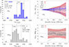 |
Fig. 8. Same as Figure 7, but for the 235U (top) and 239Pu (bottom) nuclide concentrations. |
| In the text | |
|
Fig. 9. Evolution of reaction rates as a function of burnup for relevant actinides for the assembly benchmark. |
| In the text | |
|
Fig. 10. Evolution of concentrations as a function of burnup for minor actinides for the assembly benchmark. |
| In the text | |
|
Fig. 11. Evolution of concentrations as a function of burnup for relevant fission products for the assembly benchmark. |
| In the text | |
|
Fig. 12. Evolution of the 241Am concentrations from EOL to the cooling time of 7970 days, from the assembly benchmark. Same relative x-scale is used in both histograms. |
| In the text | |
|
Fig. 13. Histograms from participants’ values for the 11 most important decay heat contributors for the cooling time corresponding to the first decay heat measurement DH1 (5823 days). X-scales: contribution to the total decay heat. Bottom right: histogram of the C/E values for the DH1. |
| In the text | |
|
Fig. 14. Relative differences between calculated and measured decay heat for the pincell benchmark. Experimental uncertainties are indicated in solid black curves. |
| In the text | |
|
Fig. 15. Relative differences between calculated and measured decay heat for the assembly benchmark. Experimental uncertainties are indicated in solid black curves. |
| In the text | |
Current usage metrics show cumulative count of Article Views (full-text article views including HTML views, PDF and ePub downloads, according to the available data) and Abstracts Views on Vision4Press platform.
Data correspond to usage on the plateform after 2015. The current usage metrics is available 48-96 hours after online publication and is updated daily on week days.
Initial download of the metrics may take a while.