


| Issue |
EPJ Nuclear Sci. Technol.
Volume 12, 2026
|
|
|---|---|---|
| Article Number | 19 | |
| Number of page(s) | 19 | |
| DOI | https://doi.org/10.1051/epjn/2026009 | |
| Published online | 16 June 2026 | |
https://doi.org/10.1051/epjn/2026009
Regular Article
Bias estimation for irradiated assembly reactivity decrement and burnup
1
Reactor Physics and Thermal Hydraulic Laboratory, Paul Scherrer Institut, Villigen, Switzerland
2
National Cooperative for the Disposal of Radioactive Waste, Nagra, Wettingen, Switzerland
* e-mail: This email address is being protected from spambots. You need JavaScript enabled to view it.
Received:
10
January
2026
Received in final form:
26
March
2026
Accepted:
17
April
2026
Published online: 16 June 2026
Abstract
In this paper, we are estimating biases for the reactivity decrement and burnup of irradiated fuel assemblies, based on differences between measured and calculated local in-core power measurements (flux maps). The simulations are performed with validated CASMO5 and SIMULATE5 cycle follow-up models for three Pressurized Water Reactor (PWR) cores. A total of more than 70 cycles of operation and 1000 in-core flux maps at various core burnup steps are used, including both UO2 and MOX fuel assemblies, as well as UO2 alone, with relatively high assembly average burnup at the end of life (greater than 60 MWd/kg). The effect of nuclear data uncertainties is also calculated and quantified on both bias types. The main findings are that while the burnup biases are globally constant as a function of the assembly burnup, the bias for the reactivity decrement tends to increase, both in terms of average values and tolerance intervals.
© D. Rochman et al., Published by EDP Sciences, 2026
 This is an Open Access article distributed under the terms of the Creative Commons Attribution License (https://creativecommons.org/licenses/by/4.0), which permits unrestricted use, distribution, and reproduction in any medium, provided the original work is properly cited.
1. Introduction
Core simulators are nowadays very powerful tools to predict the evolution of various quantities of reactor cores under normal conditions, from the neutronics aspects coupled with thermal hydraulic behavior. They can for instance be used as predictive tools prior the start of a reactor cycle for checking the compliance of a loading scheme with a number of safety parameters, for online monitoring, or for post-cycle verification and validation with respect to in-core measurements (for instance boron concentration or derived three dimensional power distributions). It is normal practice that such simulations are nowadays performed for all power reactors, using different codes such as SIMULATE, Artemis, or COCAGNE [1–3]. Apart from calculating quantities of interest for the reactor safety, core simulators, possibly combined with other codes, can also provide different important parameters for the back-end of the fuel cycle, such as assembly burnup, decay heat or nuclide concentrations. These are of high relevance for the characterization of spent nuclear fuel (SNF, also called Used Nuclear Fuel, or UNF), the design and safety of storage facilities, the SNF transport, their reprocessing or final disposal. Not only values integrated over the whole assembly can be obtained, but also local ones, at the dimension of the simulation nodes, for instance for fuel rod segment with several tens of centimeters high. Such information at the level of a few fuel pellets is of importance in the criticality-safety calculations for fuel storage or transport in cask and canister (see for instance Refs. [4–6] for the impact of the radial and axial profiles due to irradiation conditions).
The predictive capabilities of the core simulators for cycle, irradiated assemblies and SNF quantities rely on a number of theoretical calculations (e.g. neutron transport and diffusion theories), design models (assemblies, reflectors), irradiation histories (such as for the cycle of interest, as well as for past fuel assembly history) and finally computational and numerical methods allowing to provide precise answers in a reasonable amount of time. The quality of such simulations can be checked by comparing measured and calculated quantities, for instance with ex-core dose detectors, start-up tests, boron concentration as a function of cycle burnup, and in-core power detectors for various three dimensional locations and cycle steps [7–9]. Note that often the calculated quantity is not directly measured, as for in-core power, but is rather derived from absolute fission rate measurements. In a simplified manner, these values can be compared in terms of C/E or C-E, C being the calculated quantity and E the measured (or derived) one. A number of examples for this type of validation are published, see for instance Reference [10] and figure 1, or references [11–13].
Calculated average reactivity decrement biases based on PWR Hot Full Power. Values are given in pcm. Burnup values represent the center of the bins, with a width of 10 MWd/kg. See text for the definition of mixed cycles.
Calculated average burnup biases based on PWR Hot Full Power. Values are given in % of burnup. The value in italics is obtained with a low number of assemblies.
Such validation work is naturally of high importance for the estimation of reactor quantities during operation (local power, peaking factors, reactivity, boron concentration), but also for quantities which are relevant for the back-end of the fuel cycle: estimation of nuclide concentrations, their spatial distribution, assembly and local decay heat, and also assembly and local burnup. It is understandable that a difference between C and E for the power at a specific position in the core and at a given cycle time step (such difference is referred to as a bias) can be translated in an over- or under-estimation of the reactivity or burnup (for a specific assembly or assembly segment). The origin of such bias can be multiple: error in the measurement, inadequate model assumptions, approximations in the irradiation history or error (and approximations) in physics models and their inputs (such as nuclear data). Such biases for the neutron multiplication factor (keff or k∞) and burnup need to be taken into account for the validation of the simulation procedure itself, but also they need to be provided with the characterization of SNF.
In the present work, we propose to evaluate the biases on the assembly reactivity decrement and burnup based on the difference between E and C from power distributions. Such approach is not new and was extensively presented in references [12–15] with realistic examples. The term reactivity decrement corresponds to the change of k∞ with specific burnup, as described in Appendix A. The added value of the present study is the application of the method to different reactors, different fuel types (both UO2 and MOX, contrary to the previous references where no MOX fuel is used) and high assembly burnup values. The outcomes of the work are estimated values of the mean biases and tolerance intervals for the changes in k∞ (reactivity decrement) and burnup, as a function of the burnup of groups of similar assemblies (in the following, the term “sub-batch” will be used and represents a group of assemblies having similar characteristics, such as geometry, initial fuel content, and irradiation history, to follow the nomenclature of Refs. [12, 13]). Details for the considered cases (reactor cores and measurements) and for the method are presented in the next sections. The main results of this study are presented beforehand in Table 1 for the biases on reactivity decrement and in Table 2 for the burnup biases. Finer burnup bins and tolerance (as well as prediction) intervals are presented later in the paper. The analyzed cycles can contain both UO2 and MOX fuels (being mixed cycles) or UO2 fuel only.
The present estimation of biases for reactivity decrement and burnup will help for the characterization of the SNF, potentially providing uncertainties used for criticality-safety calculations of transport casks or storage canisters. It should also be mentioned that the current work is part of an ongoing research activity, based on a set of models and code versions which are not used for reference core licensing or core follow-up validation.
A number of specific terms are used in the present study, and to clarify their meaning, they are described in Appendix A. Their definition will not be repeated in the main sections of this article.
Considered plants, cycles and fuel enrichments (averaged over the active part of the fuel). For PWR1, data represent the combination of two similar units. The term “initial” corresponds to “unirradiated”.
Number of detectors in each considered core. The last line corresponds to the total number of measurements over all considered cycles (for PWR1, the measurements represent the sum for both sister units).
Simulation codes and versions for the comparison between calculated and measured power maps used in the present study (see text for details).
2. Studied cases
The reactor cores, cycles, fuel types used in the present work were presented in an initial study dedicated to analyze the difference between measured (E) and calculated (C) three-dimensional power maps, see reference [16]. In total, more than 977 000 values of E and C were compared and analyzed, coming from five Light Water Reactors (LWR). In the present study, a subset of these LWRs is considered, being three Pressurized Water Reactor cores (among which two are sister units, combined into the name of PWR1, and a third one named PWR3) and one Boiling Water Reactor (BWR), as presented in the next sections. The use of the BWR case is presented in this work as an example, and is not part of the main result of this study. The reasons are presented in Section 3.1, and lie mainly in potentially higher sources of approximations for BWR irradiation conditions, compared to the PWR ones. Such values were obtained for different fuel types (UO2 and MOX), various enrichments and core burnup values. For each cycle, core follow-up calculations were performed with different versions of CASMO5 and SIMULATE5. Details are provided in the following sections.
2.1. Plants, cycles and measurements
As mentioned, data from one BWR and three PWRs with a number of cycles and assembly information were considered in this study, and some details are provided in Table 3. For 235U initial enrichment higher than 5.0%, the assemblies contain a specific amount of 236U. Only in the case of the BWR, experimental data from the first starting reactor cycle are used, whereas for the other ones, the analysis is based on later cycles. Among the PWRs, as previously mentioned, two are sister units, having similar loading patterns and cycle strategies. The considered cycles contained different assembly geometries, with various cases for the BWRs, and more limited sets for the PWRs. More than 75% of PWR cycles contained different numbers of MOX assemblies.
As mentioned in the introduction, in-core measurement systems are used to provide axial and radial power distributions within the reactor core (see Ref. [16] for more details). Depending on the reactor type, different measurement systems can be used inside the core: fixed, movable, or both; Table 4 provides the number of measurements considered for each core type.
2.2. Cycle validation
All cycles and all plants were systematically analyzed with the same set of simulation codes, being CASMO5 and SIMULATE5 [1, 17]. Depending on the plant, different versions of these codes were used, as presented in Table 5, due to the validation scheme in place. Note that these validated models in combination with codes and versions are not part of core cycle analysis potentially used for regulatory purposes. It was observed that changes in code versions had minor or negligible impacts on the quantities of interest. CASMO5 is a deterministic lattice physics code, routinely used to produce, among other quantities, macroscopic cross sections (in the form of matrices) given the characteristics of a specific assembly design. CMSLINK5 is a utility code to process the output of CASMO5 and create a library suitable for SIMULATE5. SIMULATE5 is a core simulator using the information from various cycles (cycle length, irradiation history, reactor power, thermo-hydraulic data) and CASMO5 data matrices to produce various observables, such as three-dimensional power, reactivity or burnup distributions. The nuclear data library ENDF/B-VII.1 was used for the present study, as provided with the mentioned codes, which also used the JENDL-4.0 evaluation for 239Pu. Finally, the utility codes S3CORE and S3POST allow to compare the C and E for the local power, for different locations in the core, or integrated over various quantities. In reference [16], different code versions were compared, and in the present study, only the cases corresponding to SIMULATE5 are considered. Once the outliers were removed (based on detector locations, as explained in the previous reference) and considering cycle burnup larger than 0.2 GWd/t, a smaller number of experimental values were considered for the reactors of interest (close to 826 000). Results are usually expressed in terms of root mean square (rms) for the (E-C)/E distributions, as presented in Table 6. Different quantities can be extracted based on the E-C values, such as standard deviations or other moments of the distributions, but for simplicity, only the mean and rms are presented here. These values summarize the validation of the models and simulation tools and detailed values as a function of cycles, positions and other quantities can be found in Reference [16]. As observed, the mean and rms values vary from one plant to another, with the smallest rms obtained for the BWR reactor. Reasons for larger values for the PWR cases were presented in the previous reference, being mainly linked to the reflector and detector modeling.
Differences expressed in Table 6 are at the origin of the estimation of biases on assembly burnup and reactivity decrement, as presented in the following. In this respect, other plants and other validation methods can also modify bias values, as biases from References [12, 13] indicate (see also Tab. 1).
3. Estimation of reactivity decrement and burnup biases
The validation results for the different reactor cores and cycles presented in the previous section represent the starting point for the estimation of the assembly reactivity decrement (and burnup) biases. As explained in the following, similar assemblies are grouped together and biases are derived for such groups rather than for individual assemblies (groups of similar assemblies are later called “sub-batches”). As indicated, the present study is based on the code SIMULATE5, but due to the high number of similar calculations required, a special SIMULATE5 version was obtained from the Studsvik company, version 2.01.00_BASE. This version differs mainly from the one used for validation due to the possibility of varying the burnup value for assembly sub-batches (with a factor called Ma in the following sections) and the automation of the comparison between calculated and measured power maps with the new sub-batch burnup.
3.1. General method
The estimation of the reactivity decrement biases for groups (or sub-batches) of assemblies is based on comparisons between the calculated and measured power maps. The same applies for the burnup bias. The term “measured power maps” is deliberately not precise: power values are not directly measured, but derived from local reaction rate measurements. For simplicity, we will use this term in the following. For every reactor cycle, new assembly types are modeled with CASMO5, providing various quantities as a function of burnup, temperature, boron concentration and other parameters to the core simulator SIMULATE5. SIMULATE5 calculates then other quantities related to the considered cycle (length, core and assembly burnup, peaking factors, etc.). Validation of such modeling is performed by comparing, among other quantities, calculated and measured power maps, and the deviations between both maps are used to quantify the quality of the models (and associated methods and assumptions).
As detailed in reference [13], differences between calculated and measured values can originate from many approximations, among which: errors and uncertainties in measured reaction rates, errors in SIMULATE5 methods, in the core configuration (fuel characteristics, reactor operating conditions), and possibly errors in CASMO5 (microscopic cross sections, calculated nuclide concentrations as a function of burnup). The specific errors in CASMO5 can induce biased nuclide concentrations as a function of assembly burnup, as well as biased assembly and local burnup values in the downstream calculations with the core simulator, and with codes dealing with spent fuel quantities. If a specific cross section is too high compared to its real value, it can potentially induce increasing biases for specific nuclide concentrations, as well as for the assembly burnup. Similarly, an error in the computation of nuclide concentrations (for instance in the use of the Bateman equation or in the radial distribution) can also increase the bias for the assembly burnup.
In the present approach, all the possible sources of errors are treated together, through an iterative search for a more appropriate sub-batch reactivity effect. Such search is performed by modifying the (assembly) sub-batch burnup value at the beginning of the considered cycle, multiplying the assembly sub-batch burnup value by Ma, leading to a different sub-batch reactivity effect and by estimating its impact on core calculations with SIMULATE5. If the new sub-batch reactivity effect leads to a better agreement with measured power maps, then the difference between the original and new k∞ is considered as a bias on reactivity decrement (at a given sub-batch burnup). If no better agreement is obtained, then the bias is considered null. An example of such comparison is presented in Figure 1, corresponding to k∞ values at a specific state point within the considered cycle. In this example, the considered sub-batch of assemblies is represented with red squares, whereas the other assembly sub-batches are in white squares. The number of sub-batch per cycle typically vary from 4 to 10, depending on the considered reactor core and cycle. The locations of reaction rate detectors, from which measured power maps are derived, are indicated with crosses. The dimensions of the core, the number of assemblies, detector and sub-batch locations are simply representative of a typical PWR. As previously indicated, the comparison between measured and calculated power maps, for a specific core burnup (or integrated over all cycle step points for which measurements were performed, typically once a month) is often expressed in terms of rms. In the presented case, the original sub-batch burnup (with Ma = 1) has led to a rms value of 0.9% (the comparison was performed with two-dimensional (2D) power maps, i.e. integrated over vertical positions, but such comparison can also be performed for local measurements, leading to three-dimensional comparisons). Variations of Ma values lead to different rms values, as plotted at the bottom of Figure 1. Ma is varied from 0.85 to 1.15, with steps of 0.01. In this example, a smaller rms (indicating a better agreement between calculated and measured power maps) is obtained for Ma = 1.02. In this simple example, the difference of k∞ (for instance in pcm) between the sub-batch with Ma = 1.00 and the sub-batch with Ma = 1.02 is considered as the reactivity decrement bias. For Ma = 1.00, the k∞ provided by SIMULATE5 for this sub-batch is 0.99801, and for Ma = 1.02, the k∞ is 0.99468, leading to a bias of 0.99468 − 0.99801 = −333 pcm. Regarding the bias on the sub-batch burnup, a difference of Ma = 1.02 is obtained, translating into a difference of 2% of burnup. Naturally these biases are obtained for a specific core burnup, corresponding to a specific sub-batch burnup (being 27.3 MWd/kg in this case). By repeating this approach for all measurements as a function of core burnup (and for different cycles, and possibly cores), one can obtain the evolution of the bias as a function of the assembly sub-batch burnup.
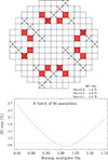 |
Fig. 1. Top: example for a representative core and cycle, with detector locations (crosses) and assembly sub-batch positions of interest (red squared). Bottom: variation of the 2D rms value as a function of the sub-batch burnup multiplier Ma (for a specific sub-batch of 16 similar assemblies). |
This example allows to understand the general method in a simplistic manner. As presented in the following, some additional constraints are added, leading to a more realistic approach.
3.2. Representative one sub-batch iterative method
The approach detailed in the previous paragraph is then generalized. For a given sub-batch of assemblies, all cycles concerned are considered, usually being a succession of 3–5 cycles. In each successive cycle, the sub-batch burnup is increasing, for instance allowing to find the adequate Ma factor for a range of burnup from low values (less than 5 MWd/kg) up to higher values (such as 50 or 60 MWd/kg). An example for a PWR is presented in Figure 2. In this figure, a sub-batch of assemblies used in 5 cycles is represented, with different colors for each cycle. For a specific cycle, measurements are performed at about 10 burnup steps (or state points), and for each step, a value of Ma is iteratively varied at the beginning of the cycle (the impact on the rms value due to the variation of the Ma factors are plotted with lines in the figure). In this simplistic example, the k∞ of this unique sub-batch is modified, whereas the effect of other sub-batches are not changed (Ma = 1.00 for other assemblies).
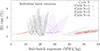 |
Fig. 2. Variation of the 2D rms value as a function of the average sub-batch burnup. Each color is for a different cycle, and each curve represents the variation of the rms at a specific state point during the cycle (due to the variations of Ma). Dots indicate the rms value for Ma = 1.00. |
The observed shapes of the curves are typical and mainly depend on the average sub-batch burnup and the location of the sub-batch relatively to the locations of the in-core detectors. For the last cycle, where the sub-batch burnup is on average high compared to the ones from other sub-batches, variations of the sub-batch burnup have less impact on the 2D rms for power densities due to the low sub-batch reactivity effect (corresponding to low sensitivity). Consequently, strong changes in burnup values are needed to impact rms values. For the first and last cycles, the imposed variations on Ma are not systematic enough to find a minimum for the rms, according to a parabolic behavior. For the very low or high burnup values, no parabolic minimum is found and the maximum of Ma = 1.15 (or minima of 0.85) can be accepted as the minimum from the linear variation of the rms. As Ma is a direct multiplier of the sub-batch burnup, extreme Ma values will lead to strong absolute burnup variation for the last cycle, and small burnup (and also reactivity effect) variation for the first cycle: considering one of the brown lines in Figure 2 (for the cycle N + 4), the range of burnup variation is about 0.85 × 52 MWd/kg to 1.15 × 52 MWd/kg, corresponding to 44.2–59.8 MWd/kg, or a variation of k∞ of 8000 pcm; for one of the red lines of cycle N, the range of burnup is this time 0.85 × 5 to 1.15 × 5 (or 4.25–5.75 MWd/kg), sensibly smaller than for the case of high burnup (the corresponding change of k∞ is only 1500 pcm). In between these two extreme variations lies the middle-range variation. Two overlapping effects can be observed: on the one hand the reactivity variability is higher for smaller burnup, and on the other hand the optimal Ma is smaller for smaller burnup. The sum of the effects leads to a larger bias for the reactivity decrement, as defined in Appendix A, and in a general manner, the reactivity bias will tend to increase with burnup.
3.3. Realistic multi sub-batch iterative method
This simple previous example allows to understand the expected trend of bias for the reactivity decrement: low at low burnup, and higher with increasing burnup values. Additionally, in order to mitigate the effect of a single sub-batch of assemblies in the variation of the rms values, the method is applied to a large number of sub-batches at once: e.g. for a single state point of a cycle, values of Ma are simultaneously and independently varied for 5–10 sub-batches at once. This allows to distribute the impact of rms variations over many assembly sub-batches at once, effectively lowering the impact of a single sub-batch. This represents the first difference between the above example and the realistic application of the method. A second difference concerns the number of iterative search to minimize rms values. Figure 2 represents the results based on a single search: the minimum in rms is found by varying Ma once. In the following, this procedure is applied in an iterative manner: each search (iteration) is based on a limited variation of Ma (a maximum change of 0.02 per iteration is allowed and in practice, steps of 0.01 are implemented), and the total number of iteration is arbitrary set to 8 (to reach variations of ±0.15). The iterative approach is implemented to solve a local minimization problem. Finally, the considered rms values are for the three-dimensional data (3D) and not the 2D values. This leads to small differences, but is perceived to allow comparisons on the actual measurements, and not values averaged over axial positions. An example of the application of the method is presented in Figure 3 for selected sub-batch k∞ effect for a specific cycle. One can observe that the bias is increasing with the burnup, as previously explained. In the original reference describing the method (Ref. [13]), the bias is described as heteroscedastic, meaning that the standard deviation of the distribution is non constant as a function of burnup (mainly due to the fact that the considered measurements are less sensitive for higher burnup). As presented in Section 4, such characteristic is also observed in the present case, and considering all cycles and all assembly sub-batches, the bias distribution will likely have a larger standard deviation at high burnup than at low burnup. One can also observe that the bias values seem to be distributed following linear functions with sub-batch burnup (with a positive slope in the presented cases). As explained in the previously mentioned reference, such behavior is expected due to the similarity of the assembly types (fuel and geometry designs), as well as from the method applied: Ma steps of 0.01 are applied, leading to reactivity changes following a “discrete-like step function”. As a conclusion, the repetition of this approach for a large number of sub-batches and cycles will lead to a statistical distribution of reactivity biases, from which averages and tolerance intervals can be extracted.
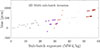 |
Fig. 3. Example of reactivity decrement biases as a function of the sub-batch burnup. The iterative search for minimizing the 3D rms is applied to many sub-batches at once. Colors correspond to different assembly sub-batches. |
Similarly, biases for the burnup of the assembly sub-batch can be obtained. A new minimum in the rms values (as plotted in Fig. 2) corresponds also a new assembly burnup value. In the example of the first state point of the cycle N + 1 (black curve), the k∞ bias is −100 pcm. The minimum in the rms curve was obtained for Ma = 0.990, corresponding to a sub-batch burnup of 12.9 MWd/kg, whereas the original burnup value was 1% higher. In this case, this difference is also interpreted as a burnup bias of 1% (for this specific assembly sub-batch and state point). As for the reactivity decrement bias, repeating this process for all assembly sub-batches and cycles will provide an average sub-batch burnup and quantities such as tolerance intervals.
3.4. Drawbacks and advantages of the method
The main advantage of this method is to allow linking measured power maps obtained in core follow-up studies with potential reactivity decrement and burnup biases. Same simulation codes are used (CASMO5 and SIMULATE5), taking advantage of hundreds of thousands of measurements within cycles and on burned fuel assemblies. As often noticed, existing criticality benchmarks, used for the validation of various neutron transport codes, are only available for fresh fuel (see the ICSBEP compilation and evaluation of benchmarks [18]). There is definitively a lack of criticality validation with spent nuclear fuel, and the present approach partly addresses this need (other recent publications were also devoted to fill this gap, such as Ref. [7]).
A number of drawbacks are nevertheless attached to the present method. The main one consists in assuming that all differences between measured and calculated power maps are linked to the reactivity effect (as calculated by CASMO5). It is known that related sources of discrepancies can come from measurement errors, detector modeling, physics model in the core simulator, cross sections, calculated nuclide concentrations as a function of the assembly burnup, and imperfect knowledge of the irradiation conditions. Consequently, the calculated biases on reactivity decrement and burnup in the present method are possibly overestimated. This drawback is not exclusive to the present work, but also applies to reference [10]. Some of the other sources of uncertainties can be assessed with different calculation methods, for instance using a different simulator core to estimate the impact of the physics model, or sampling the experimental data within their uncertainties to estimate the effect of measurements. Such estimations are nevertheless not in the scope of the present study.
Performing individual adjustments for each sub-batch of assemblies or global adjustments for groups of sub-batches would certainly lead to different results. Only individual adjustments are performed in the present work, assuming the independence of sub-batches. This assumption needs to be checked and the impact on the minimization of the rms should further be investigated.
Additionally, a number of parameters were assigned in this study, which can influence the results: selection of 2D or 3D power maps, grouping of similar assemblies in sub-batches, iteration method and numbers, as well as the range of the burnup multiplier Ma. It will be shown in the following that these parameters actually do not affect the results in a significant way.
Different validation efforts, based for instance on sample Post Irradiation Examination for pellet-size samples or assemblies [19], for core cold critical measurements, or on hot zero power conditions [7] may indicate different biases for reactivity. Finally, the results presented in the following are case dependent. Biases are obtained with the described method, using a specific set of measurements and based on particular core models and codes. These results cannot be considered as general for all LWRs, but are mostly relevant for the present combination of codes, models, and experimental data. They are nevertheless an example of existing, or calculated, biases, and can therefore be compared with other available examples.
4. Results
This section will present the main findings based on the LWR cases from Table 6, the codes presented in Table 5 and the method described in Section 3. Apart from simple averages and standard deviations, intervals and limits are also calculated. Their definition can be found in Appendix A. Results will be presented as a function of core and fuel types in the following sections, with corresponding tabulated values in Appendix B.
4.1. Determination of burnup groups
The calculated burnup values for the assembly sub-batches are continuous values. Low values of assembly burnup correspond to the lower values at which an in-core measurement is recorded with fresh sub-batches, typically being smaller than a few MWd/kg. Similarly, the highest values correspond to sub-batch burnup values at which the last cycle in-core measurements are performed, close to the end-of-life for the assembly sub-batch, typically above 50 MWd/kg. Details of the assembly characteristics can be found in reference [16]; initial enrichments are presented in Table 3.
In between these extreme burnup values, all possible sub-batch burnup values can be obtained, and it was decided to group them into burnup bins. The definition of the bins is based on having an optimum bin population following the maximum of the jackknife likelihood [20]. Therefore different burnup bins are obtained for the BWR, PWR1 and PWR3 cases, and also for the UO2 and MOX fuel types. This procedure leads for instance to 21 burnup groups for the UO2 fuel of the PWR1 (from 0.1 to 59.7 MWd/kg) and 13 groups for the UO2 fuel of the PWR3 (from 0.3 to 63.6 MWd/kg). Such burnup groups will be used in the following.
4.2. Reactivity and burnup biases for PWR cases
The values of the biases for the combined PWR cores are presented in Figures 4 (for reactivity) and 5 (for burnup). Two cases are considered in each figure: one concerning sub-batches of assemblies made of UO2 fuel only, and one with MOX fuel only. As previously mentioned, a number of studied cycles contain a mixture of UO2 and MOX assemblies, implying that the reactivity biases presented in these figures are for mixed cores, but UO2 or MOX sub-batches were separated in the figures. In addition to the individual bias values for each sub-batch at different state points and cycles (red dots), the average bias for different burnup bins is given as a bold black line. Two colored bands indicate for the same bins the tolerance and the prediction intervals. In addition, an example for a 5% reactivity decrement for a typical UO2 and MOX fuel, enriched at 4.7% in 235U and 5.0% in fissilePu, respectively, is also plotted as light red lines. These examples of reactivity decrement are also presented in reference [13] and allow an easier comparison between both studies.
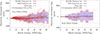 |
Fig. 4. Reactivity decrement biases considering only UO2 (left) or MOX (right) sub-batches of PWR assemblies. |
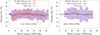 |
Fig. 5. Burnup biases considering only UO2 (left) or MOX (right) sub-batches of PWR assemblies. |
About the distribution of the sub-batch reactivity decrement biases (red dots), they globally follow the trend presented in Figure 3, confirming the heteroscedastic aspect of the bias, with values following specific lines. In total, more than 3500 values are plotted for the UO2 case, and 550 for the MOX case. For UO2, the average bias, integrated over all burnup values is less than 100 pcm (and about 3 pcm for the MOX case), which globally is relatively small, especially compared to the impact of nuclear data (see Sect. 4.5). Compared to reference [13], the UO2 biases are slightly larger (MOX cases are not analyzed in this reference); as mentioned, they are naturally dependent on the considered models, cores, cycles and measured data. It is therefore difficult to present general biases, and such values need to be linked to the considered cases. It can be noted that it is the first time that such biases are presented for MOX fuel.
Even if the average biases are small, the spread for individual sub-batches can be larger, as indicated by both the tolerance and prediction intervals. The comparison between the tolerance intervals and the example of the 5% decrement for a representative assembly indicates that for UO2, the 5% decrement is not systematically larger, especially at high burnup values. For MOX fuel, the overlap between the tolerance interval and the 5% decrement curves is more pronounced. It is nevertheless useful to note that the UO2 sub-batch population is not high for high burnup, as well as for the MOX sub-batches at all burnup bins.
Related to the reactivity decrement bias, one can also extract for the same sub-batches the burnup bias, as explained in Section 3.1. These values are presented in Figure 5. For the burnup biases, the data are more constant as a function of the sub-batch burnup, compared to the reactivity biases. No representative trend is observed for either type of fuel. The average values (independent of the sub-batch burnup) are −0.5% and +0.1% for both fuels, respectively. These small values seem to indicate a very good estimation of the sub-batch burnup, whereas the 95/95% tolerance intervals are larger, being respectively [−6.0, +5.5] and [−5.8, +5.9]%. Such intervals (being roughly ±5% to 6%) allows to consider 95% of the cases into account.
As mentioned in the introduction, other methods can be used for estimating biases for fuel assemblies, as in reference [10] based on online core monitoring. In reference [10], the burnup bias is close to 1% for all burnup values and the reactivity bias is about 250 pcm, also for all burnup values up to 55 MWd/kg. As seen in Tables 1 and 2, the average biases obtained in this work are similar: (–)1.8% for the burnup and 342 pcm for the reactivity, both between 45 and 55 MWd/kg. Contrary to reference [10], the present study also provides bias variations as a function of assembly (sub-batch) burnup, including MOX fuel. It is also helpful to extract average standard deviations from these distributions, which in the case of the UO2 fuel can be compared with the value of 0.4 MWd/kg from reference [10]. From the data presented in Figure 5, the standard deviations are close to 1 MWd/kg, for both fuel types. This value, being twice larger than for the German Konvoi study, is based on a method presenting similarities but also differences with the present work. Both studies are using CASMO5/SIMULATE, as well as measured values to extract the burnup bias. But the similarities stop there, as cycles from different plants are analyzed, with UO2 fuel versus a mixture of UO2 and MOX fuels. Additionally, the German Konvoi study is performed for one cycle, whereas the present work includes a larger number of cycles. Furthermore, the method of calculating the bias is different: in the present case, it is based on core follow-up analysis (i.e. offline), whereas online core power tracking is used in reference [10]. Finally, differences can arise from different models and model assumptions. Note that the comparison of standard deviations can be misleading, depending on the type of underlying distribution. In the present case, about 80% of the data are contained within ±1σ (one standard deviation), whereas in the case of reference [10], less than 50% of the data are within ±1σ.
Finally, one can note that differences may arise between the studied power plants in the present study (PWR1 and PWR3). Plots for individual plants are presented in Appendix C.
4.3. Reactivity decrement and burnup biases for the BWR case
The method presented and applied in the previous sections was dedicated to PWR cores, and was originally not intended to be applied to BWR systems. The main reason is that the validation of BWRs with in-core measurements depends on more (sensitive) parameters than for PWRs: knowledge of the local void coefficient or control blade movements. Consequently, the differences between the calculated and measured local power can be affected by more factors, and combining these effects under the umbrella of the bias for reactivity decrement might not be adequate anymore. It might still be interesting to compare the results of the method between BWRs and PWRs, given the above limitations. To this goal, the case of the BWR presented in Tables 3–6 was used to extract the reactivity decrement (and burnup) biases; results are presented in Figure 6. No MOX fuel was used in this BWR, so the study is limited to UO2 fuel. One can observe that the global spread of biases is similar to the PWR cases: increasing with burnup for the reactivity decrement bias, and constant or slightly increasing (in absolute value) for the burnup bias. The amplitudes of the spreads are also comparable with the PWR cores. It can be observed that the rms given in Table 6 is smaller for the BWR, which indicates better agreement between calculated and measured local power for the considered cases; this would lead to smaller biases than for the PWR cases, but as noticed, this is not observed. One of the reasons might be due to the impact of other relevant irradiation parameters influencing the current method.
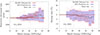 |
Fig. 6. Biases for the BWR case (left: reactivity decrement; right: burnup), similarly to Figures 4 and 5. |
4.4. Sensitivity to various parameters
The results presented in the previous sections are based on a number of selected parameters which do not directly appear in the tables or figures. These parameters and additional information is described in the following. Explicit calculated values are not presented to stay concise, but similar sensitivity results as in reference [13] are obtained. Default values and modifications are the same as in the previous reference.
-
2D or 3D reaction rates. A choice was made to use 3D reaction rate data. The study was nevertheless repeated for all the considered cores with 2D reaction rates and no significant difference was found. The advantage of using 3D data is to be as close as possible to the measured values, even if there is an important processing step to obtain power maps from reaction rate measurements.
-
Number of assemblies per sub-batch for setting sub-batch multipliers (Ma). The default value is 8 assemblies per sub-batch. This number can modify the impact that a sub-batch of assembly can have on specific rms values: with more assemblies per sub-batch, the impact will be higher. One also has to consider the size of a core and the number of similar assemblies (within in the same sub-batch). In the present case, results for two values were compared: with 8 and 12 assemblies. As previously, no significant impact was observed.
-
Number of iteration in the multi sub-batch iterative method. The selected value is 8 iterations. Higher values were tested (up to 12), increasing the calculation time without significantly changing the results.
The derived values such as the average biases and the various intervals, presented along this study, are obtained given the above default.
4.5. Uncertainties due to nuclear data
Uncertainties due to nuclear data can be obtained on the reactivity decrement and burnup biases with the method previously applied in a number of publications, see for instance references [21, 22]. The method is relatively simple: based on covariance matrices included in the nuclear data library, one can generate a set of sampled nuclear data (cross sections, emitted spectra, emitted number of neutrons) and use each set in a new CASMO5/SIMULATE5 calculation chain for all considered cycles and assembly sub-batches. The decay data were not varied, and the fission yields for the four main actinides, 235, 238U and 239, 241Pu, were varied together with other nuclear data quantities. A total of 178 isotopes are considered all together, from 1H to heavy actinides, including the most important fission products, structural elements and main actinides, based on the ENDF/B-VIII.0 covariance library. Reactions such as elastic, inelastic, fission and capture (with, in the case of the fission reaction, the number of emitted neutron per fission and its spectrum) are varied from 0 to 20 MeV, following a 19 energy-group structure. Details can be found in the mentioned references.
For each new set of perturbed nuclear data, the method presented in the previous sections is applied, leading for instance to new values of burnup biases. If one repeats this process n times, a set of n reactivity decrement and burnup biases is obtained (being n distributions similar to the one presented in Fig. 4). In total, given the available computer power, n was selected to be slightly more than 100, and the method is applied to one of the sister units of the PWR1. Uncertainties (one standard deviation) on these quantities are presented in Figures 7 and 8. Each bias value as a function of assembly sub-batch burnup is presented with an uncertainty bar (orange vertical bars in the figures), being on the average 280 and 110 pcm for the UO2 and MOX fuel reactivities, respectively, and 0.7% and 1.1% for the UO2 and MOX fuel burnup, respectively. One can observe that the uncertainties are not constant with the assembly sub-batch burnup, increasing for the reactivity and decreasing for the burnup biases. Such trend was also observed in reference [21] for the burnup uncertainties and was attributed to the decreasing effect of fissile isotopes.
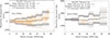 |
Fig. 7. Same as Figure 4 but for the PWR1 only (UO2 on the left and MOX on the right). Uncertainties, presented as vertical bars (1σ), are due to nuclear data. See text for details. |
The 95/95% tolerance intervals are also represented: for each of the n sets of calculations, a specific tolerance interval is obtained (gray steps in the figures), due to the variations of the single biases (orange dots). The average (and nominal, i.e. without the variation of nuclear data) tolerance intervals are also indicated with blue (and black) steps. Similarly, the figures present with the same colors the mean and nominal biases. The impact of nuclear data on the mean biases and tolerance intervals is not negligible (observed in the spread of the gray curves). The MOX cases present stronger variations as there is less fuel assemblies than for the UO2 cases, and tolerance intervals for sampled nuclear data can cross the reactivity 5% decrement which is represented in the figures. But mean (blue steps) tolerance intervals are mostly within such 5% limits. For the burnup biases, the impact of nuclear data also increases such intervals, as one can observe from the sampled gray steps presented in Figure 8. The mean is also close to the values presented in Figure 5.
Different statistical quantities can be extracted from such variations of tolerance intervals: nominal, average (considering the n = 100 cases), extreme values, or other quantities such as standard deviations, etc. Concisely, one can observe that the mean and nominal values are not strongly different, implying that the effect of nuclear data on biases is not outstanding. But individual sampled cases can strongly differ from the mean values. Additional sampling would be necessary to gain confidence on the relevance of the extreme values, which is outside the scope of this study.
As a general remark on the interpretation of the nuclear data uncertainties on quantities presented in Figures 7 and 8, they represent uncertainties on biases, and are not part of biases themselves. Both quantities (bias and bias uncertainty) need to be estimated for many criticality-safety calculations, as presented in Section 6 of the ANS standard ANSI/ANS-8.24 [23].
5. Conclusion
The main outcome of this work is the estimation of the biases on reactivity decrement and burnup, for irradiated assemblies as a function of their burnup. Cases of three PWRs are considered, including UO2 and MOX fuels, from low up to high burnup values. For a number of reasons highlighted in this work, such biases can be considered conservative. The case of a BWR core is also presented for comparison’s purpose. The method used to infer such biases is based on comparison between in-core measured and calculated power maps. Results are presented in terms of average biases and tolerance intervals, and compared with values from two published references. In addition, the effect of nuclear data was quantified. From the application aspect, the estimated biases can be used as an indication of additional uncertainties in criticality-safety and for spent fuel characterization.
Tolerance intervals for the average biases were also compared to a 5% reactivity decrement of a typical UO2 or MOX assembly. It was found that generally the tolerance intervals were included within the 5% reactivity decrement, but not systematically. Such results depend on the modeling, which includes codes, core models, cycle history and nuclear data. One should therefore not apply them to other plants and draw general conclusions. In order to gain higher confidence in the biases, it is then recommended to repeat this study for different PWRs, as results are partially different among various studies. An additional verification can consist in combining the present method with other sources of information, such as validations based on Post Irradiation Examination and measurements performed at hot zero power conditions.
Funding
This research did not receive any specific funding.
Conflicts of interest
The authors declare that they have no competing interest to report.
Data availability statement
This article has no associated data generated and/or analyzed/ Data associated with this article cannot be disclosed due to legal/ethical/other reason.
Author contribution statement
All authors equally contributed to the analysis of data and writing of the paper.
Acknowledgments
This work was partly funded by the Swiss Nuclear Safety Inspectorate ENSI (H-101230) and was conducted within the framework of the STARS program. We thank Jiri Ulrich from ENSI, for his assistance and dedicated time in reading various drafts of the present paper and in guiding us for adequate formulations. We would like also to warmly thank Bahadir Tamer, Rodolfo (Mike) Ferrer, Teodosi Simeonov and Joel Rhodes from the Studsvik company. Without their continuous support and the availability of the specific SIMULATE5 version, this work would not have been possible. Discussions with D. Mennerdahl, from E Mennerdahl Systems, Sweden, helped to focus on the most relevant subjects with the most appropriate vocabulary; we are grateful for his support. Finally, we would like to thank Marcus Seidl from the PreussenElektra company for his discussion and motivating ideas, leading to the improvement of this work.
References
- T. Bahadir, S.O. Lindhal, Studsvik’s next generation nodal code SIMULATE-5, in Advances in Nuclear Fuel Management IV (ANFM 2009), Hilton Head Island, South Carolina, USA, April 12–15, 2009 (2009) [Google Scholar]
- G. Hobson, H.-W. Bolloni, K.-A. Breith, A. Dall'Osso, R. van Geemert, H. Haase, B. Hartmann, M. Leberig, D. Porsch, B. Pothet, M. Riedmann, G. Sieber, D. Tomatis, ARTEMIS core simulator: latest developments, in SNA + MC 2013 – Joint International Conference on Supercomputing in Nuclear Applications + Monte Carlo (2014), pp. 02309. https://doi.org/10.1051/snamc/201402309 [Google Scholar]
- A. Calloo, D. Couyras, F. Févotte, M. Guillo, C. Brosselard, B. Bouriquet, A. Dubois, E. Girardi, F. Hoareau, M. Fliscounakis, H. Leroyer, E. Noblat, Y. Pora, L. Plagne, A. Ponçot, N. Schwartz, COCAGNE: EDF new neutronic core code for ANDROMÈDE calculation chain, in M &C 2017 – International Conference on Mathematics & Computational Methods Applied to Nuclear Science & Engineering, Jeju, Korea, April 16–20, 2017, on USB (2017) (2017) [Google Scholar]
- A. Detkina, D. Litskevitch, A. Peakman, B. Merk, Criticality analysis for BWR spent fuel based on the burnup credit evaluation from full core simulations, Appl. Sci. 11, 1498 (2021). https://www.mdpi.com/2076-3417/11/4/1498 [Google Scholar]
- M. Kromar, A.T. Godfrey, Determination of the spent fuel decay heat with the VERA core simulator, Front. Energy Res. 10, 1046506 (2022). https://www.frontiersin.org/articles/10.3389/fenrg.2022.1046506 [CrossRef] [Google Scholar]
- D. Rochman, A. Vasiliev, H. Ferroukhi, M. Pecchia, Consistent criticality and radiation studies of Swiss spent nuclear fuel: the CS2M approach, J. Hazard. Mater. 357, 384 (2018). https://doi.org/10.1016/j.jhazmat.2018.05.041 [Google Scholar]
- L. Berry, A. Vasiliev, D. Rochman, M. Hursin, M. Frankl, H. Ferroukhi, Application of the PSI cycle check-up methodology for full-core Monte Carlo simulations verified using pin power estimates and validated for hot zero power conditions, Ann. Nucl. Energy 211, 110939 (2025). https://doi.org/10.1016/j.anucene.2024.110939 [Google Scholar]
- B. Meunier, M. Hursin, Modeling, verification and validation of multiple PWR depletion cycles with DRAGON and PARCS, Ann. Nucl. Energy 219, 111427 (2025). https://doi.org/10.1016/j.anucene.2025.111427 [Google Scholar]
- E.E. Davidson, A.T. Godfrey, K.E. Royston, T.M. Pandya, S.C. Henderson, T.M. Evans, Validation of light water reactor ex-core calculations with VERA, Nucl. Technol. 208, 794 (2022). https://doi.org/10.1080/00295450.2021.1957660 [Google Scholar]
- M. Seidl, P. Schillebeeckx, D. Rochman, Note on the potential to increase the accuracy of source term calculations for spent nuclear fuel, Front. Energy Res. 11, 1143312 (2023). https://www.frontiersin.org/articles/10.3389/fenrg.2023.1143312 [Google Scholar]
- C. Ahnert, J.M. Aragones, F. Merino, V.K. Jain, V. Jagannathan, R.P. Jain, R.D.S. Yadav, M. Matausek, N. Marinkovic, E.Z. Mueller, G. Ball, D.L. Vogel, H. Ras, B. Petrovic, T. Smuc, N. Urli, M. Turgut, T. Turker, S. Taylan, A. Aytekin, U. Adalioglu, D. Pevec, In-core fuel management code package validation for PWRs. Technical Report, TECDOC-815, IAEA, Vienna, Austria, 1995 [Google Scholar]
- K.S. Smith, S. Tarves, T. Bahadir, R. Ferrer, Benchmarks for quantifying fuel reactivity depletion uncertainty. Technical Report, 1022909, EPRI, Palo Alto, USA, 2011 [Google Scholar]
- S. Tarves, T. Bahadir, R. Ferrer, Benchmarks for quantifying fuel reactivity depletion uncertainty – Revision 1. Technical Report, 3002010613, EPRI, Palo Alto, USA, 2017 [Google Scholar]
- E. Sykora, Testing the EPRI reactivity depletion decrement uncertainty methods. Technical Report, Master of Science in Nuclear Science and Engineering, Massachusetts Institute of Technology, USA, 2015. https://dspace.mit.edu/bitstream/handle/1721.1/103653/953277565-MIT.pdf [Google Scholar]
- V.N. Kucukboyaci, EPRI depletion benchmark calculations using PARAGON, Ann. Nucl. Energy 81, 1 (2015). https://doi.org/10.1016/j.anucene.2015.03.010 [Google Scholar]
- D. Rochman, A. Vasiliev, H. Ferroukhi, L. Berry, Bias and uncertainty estimates for in-core LWR reaction rate distributions, EPJ/N, submitted in 2026 [Google Scholar]
- R.M. Ferrer, J.D. Rhodes, Extension of linear source MOC methodology to anisotropic scattering in CASMO5, in International Conference on Physics of Reactors (PHYSOR 2014), September 28–October 3, 2014, Kyoto, Japan, no. JAEA-Conf 2014-003 (2014). https://jopss.jaea.go.jp/search/servlet/search?5049377 [Google Scholar]
- OECD Nuclear Energy Agency, International Criticality Safety Benchmark Evaluation Project Handbook, 2020. https://www.oecd-ilibrary.org/content/data/7e0ebc50-en [Google Scholar]
- F. Michel-Sendis, I. Gauld, J. Martinez, C. Alejano, M. Bossant, D. Boulanger, O. Cabellos, V. Chrapciak, J. Conde, I. Fast, M. Gren, K. Govers, M. Gysemans, V. Hannstein, F. Havluj, M. Hennebach, G. Hordosy, G. Ilas, R. Kilger, R. Mills, D. Mountford, P. Ortego, G. Radulescu, M. Rahimi, A. Ranta-Aho, K. Rantamäki, B. Ruprecht, N. Soppera, M. Stuke, K. Suyama, S. Tittelbach, C. Tore, S.V. Winckel, A. Vasiliev, T. Watanabe, T. Yamamoto, T. Yamamoto, SFCOMPO-2.0: an OECD NEA database of spent nuclear fuel isotopic assays, reactor design specifications, and operating data, Ann. Nucl. Energy 110, 779 (2017). https://doi.org/10.1016/j.anucene.2017.07.022 [CrossRef] [Google Scholar]
- D.W. Hogg, Data analysis recipes: choosing the binning for a histogram, 2008. https://arxiv.org/abs/0807.4820 [Google Scholar]
- D. Rochman, A. Vasiliev, A. Dokhane, H. Ferroukhi, Uncertainties for Swiss LWR spent nuclear fuels due to nuclear data, EPJ Nuclear Sci. Technol. 4, 6 (2018). https://doi.org/10.1051/epjn/2018005 [CrossRef] [EDP Sciences] [Google Scholar]
- D. Rochman, A. Vasiliev, A. Dokhane, H. Ferroukhi, M. Hursin, Nuclear data uncertainties for Swiss BWR spent nuclear fuel characteristics, Eur. Phys. J. Plus 135, 233 (2020). https://link.springer.com/article/10.1140/epjp/s13360-020-00258-2 [CrossRef] [Google Scholar]
- American Nuclear Society Standards Committee Working Group ANS-8.24, Validation of Neutron Transport Methods for Nuclear Criticality Safety Calculations. Technical Report, ANSI/ANS-8.24-2017, American Nuclear Society, 2017 [Google Scholar]
Cite this article as: Dimitri A. Rochman, Alexander Vasiliev, Hakim Ferroukhi, Louis Berry. Bias estimation for irradiated assembly reactivity decrement and burnup, EPJ Nuclear Sci. Technol. 12, 19 (2026). https://doi.org/10.1051/epjn/2026009
Appendix A
Definitions of terms used in this study
A.1. General terms
In this appendix, a number of terms are explicitly defined, to improve the understanding of the results. Three statistical quantities are regularly used in tables and figures, such as:
-
95% prediction interval: this is the estimate of a bias range (in pcm) or burnup range for specific assembly sub-batch burnup values in which a future calculation will fall, with a probability of 95%, given the previous observations.
-
95% confidence interval: it corresponds to the estimation with 95% confidence that the mean value for the reactivity decrement (or burnup) bias is actually within the provided range, given a number of observations.
-
95/95% tolerance limits: it represents the limits containing 95% of a specific population, with 95% probability. It is simply obtained by adding the mean to the standard deviation times a factor dependent on the sample size. The values presented in this work correspond to a 2-sided tolerance interval, based on a Normal distribution.
In addition, other simple statistical terms are used: average and standard deviation. The average corresponds to the arithmetic mean: with n realizations of a quantity x
i
(i = 1…n), the average  is equal to
  . The standard deviation, also called 1σ, is then equal to
 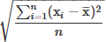 .
.
The definition of the root mean square (or rms) can be derived from the mean and standard deviation. Following the above terms, the rms can be calculated as  . It also corresponds to the sum
  . In the present study, the quantity of interest is x = C/E, with the C and E the calculated and measured local power, respectively (see Ref. [16]).
A.2. Reactivity decrement and bias
Another important term used in this study is the reactivity decrement. As indicated in references [13, 14], the reactivity decrement is defined as the difference between the k∞ for a fresh fuel assembly (at zero burnup) and the k∞ for the same assembly at a specific burnup value. If the first neutron multiplication factor is called kfresh and the second one kdepleted, the reactivity decrement Δkdecrement(BU) is defined as
 (A.1)
(A.1)
This quantity is varying as a function of the assembly burnup (BU), and is relative to a specific assembly (with its initial fuel enrichment, design and irradiation history). An example is provided in Figure 4, where such Δkdecrement(BU) is presented as red lines, for the case of a PWR assembly, with 4.7% initial enrichment in 235U. In this example, a simple irradiation history is considered, leading to a regular decrease of k∞ as a function of the assembly burnup.
The values of kfresh and kdepleted are calculated in the present case with the codes CASMO5 and SIMULATE5, as described in Section 3, based on the nominal perturbation factor Ma = 1 (see Sect. 3.1). Ma is a perturbation factor applied to the assembly burnup value BU, and as presented in Figure 1, variations of Ma leads to variations of the rms values. One can then define the reactivity decrement with an additional variable: Δkdecrement(BU, Ma):
 (A.2)
(A.2)
and depending on the value of Ma, the reactivity decrement can change. As presented in Figure 1, there might exist a certain value of Ma which minimizes the rms (i.e. δrms(Ma)/δMa = 0), called Ma’ (see Sect. 3.2 for the definition of Ma’ if the rms does not present a minimum).
Based on the value of Ma’, the bias on the reactivity decrement can be calculated as:
 (A.3)
(A.3)
Simplifying the previous equation leads to the following definition for the bias on the reactivity decrement B(BU,Ma’):
 (A.4)
(A.4)
B(BU,Ma’) is calculated at given burnup value (BU), for which the experimental values E exist, and for a specific Ma’. Such definition is the one used for Figures 3, 4, 6, 7, C.1, C.2, and in Table 1.
A.3. Burnup bias for sub-batches of assemblies
The value of the burnup multiplication factor leading to the minimization of the rms, called Ma’, enters in the definition of the bias on the reactivity decrement as indicated in equation (A.4). Consequently, one can consider the value of Ma’ as the bias on the assembly (sub-batch) burnup. This value is dimensionless (e.g. 0.99, or 1.01) but can be expressed in terms of MWd/kg by calculating |1 − Ma′|×BU, with the burnup value BU corresponding to the assembly burnup, or more precisely to the burnup of the assembly sub-batch. Such definition is used for the calculating the biases as plotted in Figures 5, 6, 8, C.3, C.4, and in Table 2.
Appendix B
Tabulated values for PWR and BWR cases
Bias values for the reactivity decrement, in pcm, for the case PWR1+PWR3 and UO2 fuel.
Bias values for the reactivity decrement, in pcm, for the case PWR1+PWR3 and MOX fuel.
Burnup bias values in %, for the case PWR1+PWR3 and UO2 fuel.
Burnup bias values in %, for the case PWR1+PWR3 and MOX fuel.
Reactivity bias values in pcm, for the case BWR and UO2 fuel.
Burnup bias values in %, for the case BWR and UO2 fuel.
Appendix C
Plots of individual PWR plants
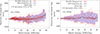 |
Fig. C.1. Reactivity decrement biases considering only UO2 batch of assemblies. Left: PWR1; right: PWR3. |
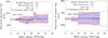 |
Fig. C.2. Reactivity decrement biases considering only MOX batch of assemblies. Left: PWR1; right: PWR3. |
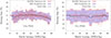 |
Fig. C.3. Burnup biases considering only UO2 batch of assemblies. Left: PWR1; right: PWR3. |
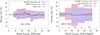 |
Fig. C.4. Burnup biases considering only MOX batch of assemblies. Numbers in italics indicate the number of batches in each bins. Left: PWR1; right: PWR3. |
All Tables
Calculated average reactivity decrement biases based on PWR Hot Full Power. Values are given in pcm. Burnup values represent the center of the bins, with a width of 10 MWd/kg. See text for the definition of mixed cycles.
Calculated average burnup biases based on PWR Hot Full Power. Values are given in % of burnup. The value in italics is obtained with a low number of assemblies.
Considered plants, cycles and fuel enrichments (averaged over the active part of the fuel). For PWR1, data represent the combination of two similar units. The term “initial” corresponds to “unirradiated”.
Number of detectors in each considered core. The last line corresponds to the total number of measurements over all considered cycles (for PWR1, the measurements represent the sum for both sister units).
Simulation codes and versions for the comparison between calculated and measured power maps used in the present study (see text for details).
Bias values for the reactivity decrement, in pcm, for the case PWR1+PWR3 and UO2 fuel.
Bias values for the reactivity decrement, in pcm, for the case PWR1+PWR3 and MOX fuel.
All Figures
|
Fig. 1. Top: example for a representative core and cycle, with detector locations (crosses) and assembly sub-batch positions of interest (red squared). Bottom: variation of the 2D rms value as a function of the sub-batch burnup multiplier Ma (for a specific sub-batch of 16 similar assemblies). |
| In the text | |
|
Fig. 2. Variation of the 2D rms value as a function of the average sub-batch burnup. Each color is for a different cycle, and each curve represents the variation of the rms at a specific state point during the cycle (due to the variations of Ma). Dots indicate the rms value for Ma = 1.00. |
| In the text | |
|
Fig. 3. Example of reactivity decrement biases as a function of the sub-batch burnup. The iterative search for minimizing the 3D rms is applied to many sub-batches at once. Colors correspond to different assembly sub-batches. |
| In the text | |
|
Fig. 4. Reactivity decrement biases considering only UO2 (left) or MOX (right) sub-batches of PWR assemblies. |
| In the text | |
|
Fig. 5. Burnup biases considering only UO2 (left) or MOX (right) sub-batches of PWR assemblies. |
| In the text | |
|
Fig. 6. Biases for the BWR case (left: reactivity decrement; right: burnup), similarly to Figures 4 and 5. |
| In the text | |
|
Fig. 7. Same as Figure 4 but for the PWR1 only (UO2 on the left and MOX on the right). Uncertainties, presented as vertical bars (1σ), are due to nuclear data. See text for details. |
| In the text | |
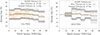 |
Fig. 8. Same as Figure 7 but for the biases on assembly sub-batch burnup. |
| In the text | |
|
Fig. C.1. Reactivity decrement biases considering only UO2 batch of assemblies. Left: PWR1; right: PWR3. |
| In the text | |
|
Fig. C.2. Reactivity decrement biases considering only MOX batch of assemblies. Left: PWR1; right: PWR3. |
| In the text | |
|
Fig. C.3. Burnup biases considering only UO2 batch of assemblies. Left: PWR1; right: PWR3. |
| In the text | |
|
Fig. C.4. Burnup biases considering only MOX batch of assemblies. Numbers in italics indicate the number of batches in each bins. Left: PWR1; right: PWR3. |
| In the text | |
Current usage metrics show cumulative count of Article Views (full-text article views including HTML views, PDF and ePub downloads, according to the available data) and Abstracts Views on Vision4Press platform.
Data correspond to usage on the plateform after 2015. The current usage metrics is available 48-96 hours after online publication and is updated daily on week days.
Initial download of the metrics may take a while.