| Issue |
EPJ Nuclear Sci. Technol.
Volume 8, 2022
|
|
|---|---|---|
| Article Number | 9 | |
| Number of page(s) | 16 | |
| DOI | https://doi.org/10.1051/epjn/2022007 | |
| Published online | 21 June 2022 | |
https://doi.org/10.1051/epjn/2022007
Regular Article
Analysis of ENRESA BWR samples: nuclide inventory and decay heat
1
Reactor Physics and Thermal hydraulic Laboratory, Paul Scherrer Institut, Villigen, Switzerland
2
Empresa Nacional de Residuos Radiactivos, ENRESA, Madrid, Spain
3
ENUSA Industrias Avanzadas S.A., S.M.E., Madrid, Spain
4
Studsvik Scandpower, Inc., Newton, Massachusetts, USA
5
National Cooperative for the Disposal of Radioactive Waste (Nagra), Wettingen, Switzerland
* e-mail: This email address is being protected from spambots. You need JavaScript enabled to view it.
Received:
16
March
2022
Received in final form:
15
April
2022
Accepted:
9
May
2022
Published online: 21 June 2022
Abstract
In this paper the isotopic compositions from 8 Boiling Water Reactor samples are analyzed following different irradiation assumptions as well as different simulation tools. These samples are part of a proprietary experimental program by a Spanish consortium, and they were obtained from a GE14 assembly irradiated in Sweden. Calculated nuclide concentrations are compared with measured ones providing biases for a selection of isotopes and samples; calculated uncertainties are also provided. Finally, the decay heat from one the sample segment is calculated and compared among the different simulation assumptions. It is shown that depending on the considered nuclear data library and modeling, different contributors affect the calculated quantities, indicating a certain level of prediction power.
© D. Rochman et al., Published by EDP Sciences, 2022
 This is an Open Access article distributed under the terms of the Creative Commons Attribution License (https://creativecommons.org/licenses/by/4.0), which permits unrestricted use, distribution, and reproduction in any medium, provided the original work is properly cited.
1 Introduction
The analysis of Post Irradiation Examination and more particularly of the isotopic composition from irradiated samples is a necessary step for estimating the performances of neutronics simulation tools such as CASMO5 or SCALE [1,2]. A large number of validation reports and journal articles can be found in the open literature as such code users are required to compare measured and calculated nuclear quantities, for instance within the framework of criticality-safety, Spent Nuclear Fuel characterization, and many others. The present work is also part of the validation of specific calculation scheme, representing the modelization of a specific irradiation environment (for instance a two- or three-dimensional assembly), the irradiation history (cycle parameters, cooling time), boundary conditions and finally the simulation tool (including neutronic transport, depletion and decay). Recently, a consistent method was applied to the Pressurized Water Rector (PWR) UO2 samples GU1 and GU3 and to the PWR MOX samples BM1 and BM3 [3–5] (similar hypothesis with respect to the simulation codes and methods, nuclear data libraries, uncertainties), allowing to compare the prediction capabilities, as well as calculated uncertainties.
To complement the previous analysis with BWR samples, the analysis of 8 BWR samples, taken from the same assembly rod, namely the so-called “ENRESA” samples is presented in this paper. They are part of a proprietary experimental program organized by a Spanish consortium, consisting of ENRESA, ENUSA and CSN, representing the Spanish nuclear waste organization, fuel vendor, and regulatory body, respectively. The isotopic measurements and details of the irradiation conditions are not publicly available and the information presented in the following is obtained from references [6–8]. The present simulations, nevertheless, are based on non public information, available within the European EURAD project, work package 8 [9], and provided by ENRESA [10]. The isotopic compositions were calculated with two different codes (CASMO5 and POLARIS), in four different simulations. For the POLARIS simulations (called POLARIS-1 and POLARIS-2 in the following), the same irradiation descriptions were used, following reference [10] for a single assembly irradiation with reflective boundary conditions. These simulations were performed by independent groups (Nagra and ENRESA/ENUSA). For the two CASMO5 simulations, called CASMO5-1 and CASMO5-2, different assumptions were considered and the simulations were also independently performed (by PSI and Studsvik). The CASMO5-1 calculations are also following reference [10] for a single assembly case, whereas the CASMO5-2 case represents an attempt to model a 3 × 3 cluster of assemblies, based on reference [10].
Results concerning comparisons between measured and calculated isotopic concentrations and calculated uncertainties, as well as a comparison between calculated decay heat values (and uncertainties) are presented in the following. Apart from helping for the validation of the mentioned codes, this work contributes to the studies performed in the European Project called EURAD, and more specifically in the work package 8, dedicated to “Spent Fuel Characterization”. This work will show that the spread of results from the four simulations also indicates differences which can be larger than the calculated uncertainties themselves.
2 The BWR samples
As mentioned in the introduction, the 8 BWR samples used in this work are from the proprietary Spanish experimental program. Despite the non-public aspect of parts of the irradiation information, all data presented in this paper are extracted from publicly-available publications, see references [6–8, 11–13], but the simulation history and measured values are obtained from the EURAD project. In the following sections, a number of details will be given, not necessary sufficient to perform the irradiation simulations.
2.1 Assembly characteristics
Measurements of the isotopic compositions were performed for the rod J8 from the GE-14 10 × 10 assembly called GN592, irradiated in Sweden, in the Forsmark Unit 3 BWR reactor, see the schematic representation in Figure 1. The assembly GN592 was made of 92 UO2 rods, including 14 part-length rods, nine rods containing Gd2O3, and seven different uranium enrichments. As indicated in the figure, natural uranium was used as blankets at the top and bottom of the assembly. The eight samples are located at six vertical positions in the J8 rod, as indicated in the figure. Such positions span over the dominant and the vanishing parts of the assembly. The segments indicated in the figure correspond to the division performed by the core simulator. For each segment, different values for the irradiation conditions are provided in reference [10]. As noticed, two segments contain each two samples (samples ENRESA-1 and -2, and ENRESA-3 and -7), allowing for testing the reproducibility and randomness of the isotopic measurements. The rod J8 was made of UO2 with an enrichment of 3.95% of 235U, without gadolinium, for all segments containing samples. The cladding is made of Zircaloy-2. Table 1 summarized the non-proprietary data for GN592 assembly parameters from reference [12]. The assembly GN592 was irradiated for five consecutive cycles (cycle 16–20) from July 24, 2000, and was discharged on May 28, 2005.
One can notice that the fuel temperature is provided at a specific burnup value. It is nevertheless recognized that the fuel temperature can vary up to a few hundred degrees as a function of the segment burnup and power [14]. These parameters were used in all the following simulations.
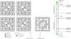 |
Fig. 1 Assembly GN592, GE-14 type, with various rod types. The rod J8 containing the 8 samples is indicated in red for the transverse view. On the right is indicated the axial sample positions. Segments in green corresponds to natural uranium [6]. |
2.2 Sample burnup values
The burnup values for the 8 samples are both provided in the EURAD document (not publicly available), and in published studies, as presented in Table 2. Samples are ordered as a function of the axial height (Note a certain difference between different references; such differences do not modify the node of interest). There are some discrepancies in the reported values, not larger than a few MWd/kgU, except for sample 4, where reference [6] report 56 MWd/kgU, whereas other values are sensibly lower. Reference [6] is in fact using the values reported in reference [10] based on the 148Nd/238U measurements. The reported uncertainty for this value is nevertheless large, or larger than for the other samples. Additionally, burnup calculations based on other Nd isotopes, 235U or239 Pu are generally lower for this sample [10]. It can be mentioned that the original report [10] indicates that the determination of sample burnup values based on actinide concentrations is less reliable for BWR than for PWR, due to the complex irradiation conditions. Values derived from gamma-scanning or 148Nd are therefore more trustful.
In the present work, the CASMO5 single assembly calculations (called CASMO5-1 in the following) are performed to match the 148Nd contents, by modifying the segment burnup to obtain an agreement for the 148Nd isotopic concentrations. Therefore, the calculated sample burnup values are in agreement with reference [6]. It is nevertheless important to note that different burnup values are obtained (and reported), based on the selected reference isotopes; it is an advantage to propose different burnup values for the same sample, but it also leads to accept a certain amount of uncertainty. In cases reported in reference [10], the spreads between burnup values, for the same sample, vary from 2.0 to 5.9% (standard deviation).
A final remark concerning samples 5 and 8 can be made. As indicated in Figure 1, these two samples are assumed to be in different nodes. This comes from the fact that they are separated by about more than 10 cm, as mentioned in Table 2. In the original report [10], samples 5 and 8 are indicated to be in the same node in one table of the report, but sample 5 is locatey close to the limit between two consecutive nodes. As these samples are located in an elevation where the gradient of the neutron flux is strong, it can have an important impact on the simulation. In the present work, these samples are either considered in different nodes (the simulations are performed with different values for the sample environment) or an average of the irradiation conditions is considered (as detailed in Sect. 3.1.3 for the Polaris-2 simulations).
Characteristics of the ENRESA samples, as found in the literature and this work (from the CASMO5-1 simulations). The axial height is measured from the bottom of the fuel rod end plug.
2.3 Measurements for isotopic concentrations
All measurements were performed at the Studsvik Nuclear Laboratory between 2006 and 2009. A large number of isotopes were measured: 68 nuclides (14 actinides and 54 fission products), as well as 21 elements for each of the eight samples. The list of 68 nuclides is found in the following of this paper, within tables and figures. In this work, only the isotopic measurements are considered, as the concentrations for the elements were not available. Various techniques of measurements were used, as presented in Table 3. The method of γ-scanning corresponds to rod-axial measurements of 137Cs gamma-rays, ICP-MS is the Inductively Coupled Plasma - Mass Spectroscopy, IDA corresponds to “Isotope Dilution Analysis / High Pressure Liquid Chromatography - Mass Spectroscopy”, and finally DRC-ICP-MS is the “Dynamic Reaction Cell / Inductively Coupled Plasma Mass Spectroscopy”. A few isotopes were measured with different techniques as indicated in the table, such as 235U, 239Pu, or 137Cs, to mention only some application-relevant isotopes. It is not possible neither useful to comment on all measured values and methods, but a few remarks can be made in specific cases.
For 235U, concentrations were obtained with the ICP-MS and IDA methods. Concentrations from IDA are generally larger than those from ICP-MS (for all but one sample), with smaller standard deviations (smaller by a factor 2–3): the average difference is about 1.7%, well within the ICP-MS uncertainties.
For 239Pu, same measurement methods as for 235U were used. Concentrations from IDA are systematically larger than those from ICP-MS, and for six samples, outside one experimental standard deviation. The average difference is about 8% between concentrations from both methods.
For 137Cs, the concentrations were obtained by means of gamma-scanning and IDA. Uncertainties are generally between 1 and 3%, and for six samples, differences between both method concentrations are larger than one standard deviation.
Additionally, a number of concentrations are provided at the end of irradiation, implying that a specific decay correction was applied to the original measured concentrations. This concerns the nuclide inventories based on gamma-scanning, and other specific cases from the IDA measurements (some Gd, Eu, Cs, Pu and Am).
Final remarks can be made for samples being very close: samples 1 and 2, and samples 3 and 7, see Figure 1 (denominated 1/2 and 3/7 in the following). As these samples are separated by about 1 cm, their nuclide concentrations are expected to be very close: differences cannot be observed from the calculation aspect (samples located in same segments), and differences between measured values should not exceed statistical variations. For a large number of important isotopes (e.g. 235,238U,239,241 Pu, 241Am, 244Cm, 137Cs), the concentrations for these samples are in agreement (within one standard deviation for the IDA method). But some discrepancies can be observed for sample 3/7 concerning 148Nd.
List of measurement methods for each isotope. See text for details.
3 Analysis of PIE
The analysis of the sample nuclide concentrations was performed by four different institutes, based on the same description of the experimental program, i.e. report reference [10]. Differences in the results, expressed in terms of C/E − 1 (C: calculated values and E: experimental values), are nevertheless observed and presented in the following. As four different simulations are performed, four different C values are obtained. It is expected that such differences in calculated concentrations arise from different interpretation and modeling of sample irradiation conditions, as well as from the different transport and depletion codes. As a recall, readers can also find different analysis in references [6–8].
As mentioned earlier, a large number of nuclide concentrations were measured, and not all results can be presented here. In the following, the comparisons will be performed for a selection of isotopes, coming from an expert choice based on the isotope relevance and experimental confidence.
3.1 Modeling
The modeling of the sample irradiation is performed following a traditional approach. Two-dimensional simulations are performed, for specific assembly segments (vertical slices), given specifications from reference [10]. The irradiation characteristics are varying with irradiation steps, for each cycle. As presented in this section, four different simulations are performed, two with CASMO5 [1], and two with POLARIS [2]. Due to the proprietary aspect of report reference [10], no details are provided for specific model parameters.
Some remarks can be applicable to all modeling options. The pin of interest, as indicated in Figure 1, is on the narrow side of assembly GN592. This location makes the pin neutronic and thermal-hydraulic environment very sensitive to the surroundings, especially the assembly across the side from the fuel rod J8 of GN592. Additionally, as the considered assemblies are of small size, the neutronic and thermal-hydraulic environment can be significantly affected by the core periphery and possibly inserted control blades. For GN592, the irradiation position for the two last cycles was close to the core periphery, but no information is available about the position of the control blades for cycle 17 and 18.
The four different simulation approach can be summarized as follows:
- –
CASMO5-1: single assembly model, reflective boundaries, adjusted burnup to fit the 148Nd measured concentrations, code version 2.03.00, with the ENDF-B/VII.1 nuclear data library,
- –
CASMO5-2: 3 × 3 assemblies model, reflective boundaries, no burnup adjustment, code version 3.02.00, with ENDF-B/VII.1,
- –
POLARIS-1: single assembly, reflective boundary, no burnup adjustment, code version 6.2.3, with the SCALE 56-group multigroup library,
- –
POLARIS-2: single assembly, reflective boundary, adjusted burnup to fit the 148Nd measured concentrations, code version 6.2.4, with the SCALE v7-252 multigroup cross section library.
3.1.1 Single-assembly CASMO5 calculations
This CASMO5 simulation is similar to the single-assembly analysis performed for the GU1, GU3 and BM1 samples. It will be referenced as CASMO5-1 in the following. The transport and depletion calculations are performed with the version 2.03 of CASMO5, using the library called “e7r1.201.586.bin”, based on the US ENDF/B-VII.1 original nuclear data library. The specificity of the neighboring assemblies are not considered, although a number of average parameters are provided in reference [10] for assemblies surrounding GN592 (not all necessary information can be found in this reference). Two-dimensional segments are modeled, as presented in Figure 1, leading to six models (for different samples), with different geometries (either dominant or vanishing parts), and different parameters such as fuel and moderator temperatures, void fraction, varying at each depletion steps over the five consecutive cycles (with downtime). For each cycle, between 10 and 15 irradiation steps are used. The nuclide concentrations are extracted at the end of the irradiation, with defined cooling steps, corresponding to the measurement periods. Similarly, a segment decay heat is calculated using the module called “SNF-Lite” from CASMO5.
Reference [10] provides the calculated sample burnup values, based on different burnup indicators for each sample (Nd isotopes, 235U and 239Pu concentrations and 137Cs gamma-scanning). In these calculations, the burnup values derived from the 148Nd concentrations are considered and burnup steps for these calculations are adjusted to reproduce these concentrations.
In the following, the results for samples ENRESA-1 to -8 are presented in Figure 2 for the nuclide concentrations, and in Figure 3 for the decay heat obtained from the segment of the ENRESA-1 sample. Additionally, tabulated C/E values are presented in Table A.2 for sample ENRESA-1.
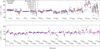 |
Fig. 2 Comparison for calculated and measured nuclide concentrations between the four types of calculations (top: actinides, bottom: fission products). In each subbox, data are ordered from left to right as a function of the sample vertical elevation. |
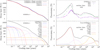 |
Fig. 3 Left: calculated decay heat for the segment containing the sample ENRESA-1. Right: calculated decay heat uncertainty for the same segment: comparison with other samples assuming same input uncertainties (top) and contributions to the total uncertainties (bottom). |
3.1.2 Multi-assembly (MxN) CASMO5 calculations
These simulations, denoted as CASMO5-2 in the text, are performed with CASMO5, version 3.02.00, and the nuclear data library “e7r1.202.586.bin”. Differences due to the code version regarding the previous simulations are expected to be small compared to the those coming from the change of modeling. The goal of this, so-called “MxN”, simulation (or multi-segment option) is to compute the sample exposure by performing burnup calculations for an entire, 3 × 3-assembly system. Examples of such approach can be found in reference [15] for the ARIANE BM1 sample, for pin power calculations of a full PWR core [16], and for bowing effects in references [17, 18].
In general, such simulation should provide more realistic boundary conditions, compared to single assembly models, for the irradiation of the assembly GN592 placed in the middle and from there for the calculation of the pin exposures. For a proper simulation, the 3 × 3 assembly material and geometry properties, 3 × 3-void distributions, 3 × 3-fuel and moderator temperatures, and control rod insertion should be provided for each burnup step, in addition to the beginning of cycle (BOC) burnups for the surrounding assemblies for each axial level. An iterative procedure is applied for each burnup step, with power density for the entire system varied until corresponding axial nodal burnup of GN592 provided in reference [10] is reached. However, reference [10] provides only limited information for the properties and the irradiation conditions of surrounding assemblies. Therefore, the analysis presented in this work were performed under several assumptions derived from the limited 3 × 3 data provided in reference [10] and the data available for assembly GN592: radially uniform, across all assemblies, void, and fuel temperature, and moderator temperature, distributions; a control rod was inserted for all samples during the irradiation in cycles 17 and 18; axially uniform BOC burnup for the surrounding side assemblies equal to assembly average, fixed pin-layout, geometry and burnup equal to 25 MWd/kgHM for the assemblies in the corners of the 3 × 3-system; reflective boundary condition for all cycles assuming inner-core position for the 3 × 3-cell. It is expected that these assumptions will impact the sample irradiation environment, and not automatically lead to the correct sample burnup. For example, for sample ENRESA-1, this procedure leads to a sample burnup of 47.9 MWd/kgU. This type of simulation, without normalization to 148Nd concentrations, approaches the isotopic evaluation from another aspect and provides an estimate for quality of the modeling with limited amount of information. It should be pointed out that, in realistic cases without measurements, the normalization to 148Nd will not be available and code performances cannot be expected to be as good as when the 148Nd concentrations are known. The impact of not normalizing the sample burnup was also presented in reference [5] for the BM1 sample and full core simulations.
3.1.3 POLARIS models
The modeling using the SCALE/POLARIS code was performed at Nagra and independently at ENUSA. In the following, results from Nagra and ENUSA will be labeled “POLARIS-1” and “POLARIS-2”, respectively.
In the case of the POLARIS-1 simulations, the calculations were performed using POLARIS from the SCALE nuclear modeling and simulation code [19] (version 6.2.3), along with the SCALE 56-group multigroup library. The decay and fission yield data are based on the ENDF/B-VII.1 nuclear data library, while the multigroup cross-section library is based primarily on ENDF/B-VII.1, along with supplementary data from the JEFF-3.0/A nuclear data library, which is recommended for generalpurpose reactor physics and LWR analysis. The assembly models in POLARIS are 2D axially symmetric models, representing a single assembly hosting the irradiated sample. The surrounding assemblies of the modeled assembly are approximated by default in Polaris using reflective boundary conditions (radially). ORIGEN is coupled to Polaris to perform the depletion and decay calculations, and therefore to simultaneously generate time-dependent isotopic concentrations, and subsequently decay heat.
The irradiation parameters, e.g., the nodal values of the void fractions, are provided in report [10]. The power densities and the void fractions at the axial locations of the samples were interpolated from the provided nodal values. Table 3.7 of reference [10] provided the nodal values of the power densities, and Table 3.9 of the same reference provided the nodal values of the void fractions. No normalization to the measured Nd isotopes was necessary.
Regarding POLARIS-2 (ENUSA) simulations, the isotopic compositions of six samples (ENUSA-1 and ENUSA-2, as well as ENUSA-3 and ENUSA-7 were analyzed together as they are very close and have the same irradiation history) were calculated using Polaris from the SCALE Code System, version 6.2.4. A two-dimensional single assembly was modeled with the exact irradiation history extracted from reference [10], including the downtimes between cycles. The SCALE v7-252 multigroup cross section library based on US ENDF-B/VII.1 nuclear data was used. The sample power at each irradiation step was calculated from the nodal burnup provided in reference [10] adjusted to the sample burnup (from the weighted average of Nd values) and divided by the irradiation time of each burnup step. For the samples that were analyzed together the nodal burnup was adjusted to the average burnup of both samples. For the ENUSA-5 sample, since it is located near the limit between nodes 22 and 23, the average history (burnup and void fraction) between both nodes are used. Additionally, the moderator density was derived from the segment void fraction. Nuclide concentrations at the measurement time were obtained from an ORIGEN decay calculation using the calculated Polaris inventory at the end of irradiation.
3.2 Comparison between measured and calculated concentrations
The comparison between some of the calculated and measured nuclide concentrations are presented in Figure 2. Such comparison is performed for a selection of isotopes, from IDA or ICP-MS with external calibration. When a specific isotope is measured with both methods, the average value is considered. Four different calculated values are presented for each isotopes, obtained from the previous models. For each isotope, the values for the eight samples are presented in the order of elevation in the rod (starting with the sample ENRESA-6 on the left of each subbox, and finishing with ENRESA-8). In the case of the POLARIS-2 calculations, not all samples were analyzed. The solid steps represent the average of the calculations and the gray bands are the calculated uncertainties (one sigma, see Tab. A.2).
In the case of actinides, the spread of C/E values is increasing for Am and Cm, as the concentrations of actinides heavier than the fresh fuel content result from many neutron captures, highly sensitive to the neutron fluence and spectrum. The calculation of the concentration of such actinides is also subject to successive cross sections biases. There is also no clear trend as a function of the sample position. The calculated values from the CASMO5-2 simulations, not normalized to the estimated burnup, is showing in general the largest deviations from the measurements. One can observe that if the average is considered (black solid line in the figure), deviations from C/E = 1 appear small for actinides up to 241Am. This covers the fact that individual calculations can strongly differ, undermining prediction power. This case is relatively similar to the validation of decay heat calculations, as presented in reference [20]: individual cases can show large deviations from C/E = 1, but their average is close to C/E = 1. Finally, one can observe that the prediction of the Cm isotopes is relatively poor, and in the case of 244Cm, calculated uncertainties do not help understanding differences between C and E (see details in Sect. 4 for the uncertainties). In the case of fission products, the trends are more case dependent. As mentioned earlier, the experimental 148Nd concentrations provided in reference [10] for samples located in the same segment can differ by up to 8%, which is an important value given that it represents many experimental standard deviations. Different 148Nd concentrations can lead to sensibly different sample burnup values, and consequently to differences in many calculated isotopic concentrations. It is interesting to compare the present results with the ones presented in reference [7] for a large number of measurements for BWR samples. Results are presented in a statistical way (with various moments of distributions) for various isotopes. The trend is similar with the present work for 99Tc, 143,145Nd, 155Gd (overestimation), 133Cs and 149Sm (underestimation), given that the eight ENRESA samples are also included in reference [7]. The observations are not similar for actinides, although 234U, 239Pu and americium isotopes also indicate similar trends.
It can be noted that in the case of the CASMO5-1 calculations and the sample ENRESA-1, the results can be strongly modified if the void fraction is artificially changed in order to fit the measured concentrations: an increase of the void fractions for all cycles helps in improving the agreement for U and Pu isotopes, at the same time.
4 Uncertainties
The estimation of the uncertainties for nuclide concentrations is performed with the single-assembly calculations using the CASMO5-1 models, as described earlier in the paper. The method consists in repeating similar CASMO5 calculations, each time with slightly different parameters. One parameter (for instance the fuel temperature) is changed at a time. After performing a number of variations, different calculated nuclide concentrations are obtained; the standard deviation of such distribution is considered as the uncertainty due to the variation of a specific input parameter. This way, uncertainties are obtained at the same time for all quantities calculated by CASMO5: nuclide concentrations as well as decay heat. Apart for the void fraction, all input parameters and their uncertainties were varied in a similar way (same method, same initial variations) for the PWR samples called GU1, GU3 and BM1, presented in references [3–5], allowing a consistent comparison of uncertainties.
4.1 Input variations
The following quantities were separately varied: nuclear data, segment void fraction, fuel and moderator temperatures, depletion steps (or segment burnup), fuel enrichment and density (together), rod radius, rod location and pitch.
In the case of nuclear data, the covariance information as provided by the nuclear data libraries was used. Three library covariances were considered: ENDF/B-VIII.0 [21], JEFF-3.3 [22] and JENDL-4.0 [23]. All cross sections, particle emission (mainly neutrons, known as nubar) and emission spectra were varied at once, according to the covariance matrices processed in 19 energy groups. The base library for the CASMO5 calculations is the ENDF/B-VII.1 library (release number e7r1.201.586.bin in CASMO5 nomenclature), and only perturbation terms were applied, using the PSI tool called SHARK-X [24, 25]. In the following, the uncertainties on the nuclide inventories and decay heat will be presented for each of the three libraries, also comparing values with the other PWR mentioned samples.
All modeling parameters were varied applying uniform distributions with the following standard deviations: 0.5% for the pitch, 0.3 mm for the rod displacement (each rod was considered independent of each other, and displacements were randomly applied for each rod at the beginning of irradiation), 0.5% for the rod radius (considering all rods independent from each other), 1% for the fuel density, together with 0.2% for the fuel enrichment (also all rods considered independent from each other), 0.25% for the depletion steps (all fully correlated for a single simulation; for instance, all burnup steps are increased by 0.1% for a specific simulation), and finally 2% for the fuel and moderator temperature (also fully correlated for a single simulation). These parameters and uncertainties were also used for GU1, GU3 and BM1. In the case of the void fraction (not applicable for PWR samples), the considered uncertainty is 35%, with a uniform distribution (as long as the void fraction is between 0 and 100%). Such variation is justified by the general difficulty to assess correct values, and by the lack of variation of the void fraction within the lattice (a single value is used for the full lattice, regardless of the radial information).
4.2 Results
Results for nuclide concentration uncertainties and decay heat uncertainties are presented from Table A.1 to A.5. As for the previous PWR samples studied, two different types of uncertainties are provided: the standard deviations coming from the sampling of model parameters and nuclear data, and so-called “expanded uncertainties”, which combined biases and the strictly speaking uncertainties [26].
Regarding the impact of nuclear data, the calculated uncertainties on nuclide inventories are among the largest compared to other variations (see Tab. A.1). This was also noted in previous studies: whereas actinides depend mainly on capture and fission cross sections, fission products are mainly influenced by fission yields, with some exceptions. Differences of the uncertainties for various libraries are also large in some cases: if they lead to similar uncertainties for actinides, fission product uncertainties can be an order of magnitude apart. This was also noticed for the other samples GU1, GU3 and BM1, and mainly comes from differences in fission yield uncertainties. It is also interesting to note that regarding the maximum uncertainties per isotope (from either library), there is no strong differences between the UO2 samples (ENRESA, GU1 and GU3). If one also compares with the UO2 sample called U1 from the proprietary LWR-PROTEUS [27], a similar conclusion can be drawn.
The impact of the void fraction is relatively important for actinides such as 235U and 239Pu, but also for a number of heavier actinides. In some cases, it is larger than the effect of other parameters, including nuclear data. This is specific to BWR, and it indicates the importance to correctly estimate the void fraction for the calculation of isotopic concentrations, but as indicated in the following, also for decay heat.
4.3 Beyond uncertainties
As mentioned in the previous section, the calculated uncertainties on the nuclide concentrations are in general not large enough to explain the disagreement between the calculated and measured concentrations. This can be seen in Table A.3, where the expanded uncertainties, taking into account the observed biases, are significantly larger than the uncertainties obtained from input variations. It was not the case for the PWR analyzed samples, possibly indicating that the modeling conditions seem more adequate for these samples. For main actinides, such as 235U and 239Pu, biases are large, as well as the expanded uncertainties, indicating a model deficiency, and (or) underestimated model uncertainties. For fission products, the observations are more diverse, but globally the same effect can be observed.
The modeling of BWR irradiation assembly is more challenging than for PWR; this was noticed in a number of publications, due to heterogeneous irradiation conditions, void and temperature effects [28–30]. Additionally, the considered rod is at the edge of the assembly, amplifying the impact of the assumption of a flat void fraction for the whole segment. Neighboring assemblies, with different burnup values, as well as the presence of a local control rod can significantly affect the neutron spectrum, especially since the considered assemblies are of small dimensions. reference [28] indicates that for the considered BWR assembly simulation, the moderator density can be as different as 15% from the average value, with extreme values up to 30%, strongly affecting actinide concentrations (235U, Pu isotopes), and specific fission products (such as Nd). In reference [29], it is concluded that the proximity of absorber blades, in the case of relatively small BWR bundle (as the one considered here), affects the distribution of the void fraction across the assembly. This reference also indicates that the effect of nuclear data on void fraction prediction is significant, with observed differences of 40% or more. reference [30] also confirms that the void fraction greatly varies within a bundle similar to the one used in the study, based on computational fluid dynamics calculations. In addition, the attempt to take into account the close assemblies with the simulation called CASMO5-2, considering the available partial information from reference [10], does not lead to improved C/E values. It indicates that key quantities were not captured by this more elaborated model, and possibly including inadequate assumptions. Additionally, using independent simulations, based on similar understanding of the irradiation conditions, indicate that isotopic concentrations are on average relatively well reproduced, but individual calculations can differ from each other. Such differences are not captured by the calculated uncertainties, but are nevertheless part of the variability of the predictions. In the present case, the differences between the four simulations can be larger than the calculated uncertainties.
5 Decay heat
The decay heat of a particular two dimensional segment can be obtained from the previous calculations by extending cooling times and requiring the specific decay heat output. It is not a measured quantity, therefore comparison and analysis can be made solely based on calculated quantities. Calculated decay heat as a function of cooling time for the assembly segment containing the sample ENRESA-1 is presented in Figure 3 left. Values from both codes CASMO5 and POLARIS are presented. The main contributors to the decay heat are also presented in Figure 3 left, obtained from the CASMO5-1 calculations. The same isotopes as for the UO2 PWR samples are observed, with different relative contributions due to different irradiation conditions: fission products generally dominate at short cooling time, and the actinide importance increases with time.
The decay heat uncertainty can be obtained following the same variations as in the case of the calculations of the nuclide concentrations. It allows to obtain consistent variations (and uncertainties) between these quantities. Additionally, as the same parameter variations were applied in the case of the mentioned PWR samples, the decay heat, in terms of Watt per ton, can directly be compared. Tabulated values for the segment containing the sample ENRESA-1 are presented in Tables A.4 and A.5, using the modeling of CASMO5-1. The impact of individual variations are presented, as well as the expanded uncertainties, taking into account the biases from the nuclide compositions. In the case of nuclear data, the decay heat uncertainties are also presented in right panel of Figure 3. The comparison of uncertainties with other PWR samples is indicating differences, due to the segment burnup, fresh fuel characteristics and irradiation conditions, but there are no strong observed variations (top of Fig. 3, and the four last columns of Tab. A.4). All uncertainties are within a factor 2, and smaller than 7%. These values represents the impact of nuclear data, coupled with the effect of varying input parameters within specific ranges, but it does not account for the nuclide concentration biases, neither for the "user effect" (different modeling strategy, considering similar sample and irradiation specifications).
The biases due to nuclide concentrations are included in the so-called expanded uncertainties, following the definition of reference [26]. Such quantities are less general than the uncertainties presented in Figure 3, as they included specific differences between measured and calculated nuclide concentrations. Values are presented in Table A.5. One can see that naturally uncertainties are increased, notably at short cooling time (up to 17% at 1 year cooling time). Similar effect can be observed for the GU1 sample, where uncertainties reach a maximum between 0.5 and 1 year (up to 23%); for GU3, the maximum is reached at 500 years (11%), and for BM1 between 1 and 3 years (65%). These values are strongly affected by the agreement between the calculated and measured isotopic contents, and are therefore extremely case dependent.
As observed in Figure 3, the calculated decay heat from the CASMO5 and POLARIS models are not identical. Such difference can be compared to the calculated uncertainties, as presented in Figure 4. The difference between the four calculations (CASMO5-1, CASMO5-2, POLARIS-1 and POLARIS-2) is expressed in terms of relative standard deviations as a function of cooling time, as presented in the figure. One can observe that such standard deviation is in general larger than the calculated uncertainties (ΔCmax from Tab. A.3). The maximum reaches almost 11% between 10 and 100 years of cooling time, and is mainly due to differences in the production of 241Am and 238Pu (almost half of the difference for each isotope at 50 years of cooling time). Such differences can originate in different nuclear data libraries, as well as in irradiation conditions. It nevertheless indicates that the impact of the modeling, not captured by the uncertainty propagation method, is in the present case more important than other quantities.
Finally, one can see the different contributions to uncertainties due to the nuclear data on the bottom of Figure 3. The same main contributing isotopes were found for the PWR UO2 samples: 134Cs, 137mBa, 244Cm, 241Am and for long-term storage (and low decay heat values): 239Pu and 240Pu. Such contributions were obtained based on the ENDF/B-VIII.0 covariance data, and as indicated in Table A.4, results can vary for different libraries. One important change concerns 134Cs, which contributes less in JEFF-3.3, and also in the SCALE library used for the POLARIS-1 calculations (uncertainties from the SCALE calculations are not presented here). In the case of the POLARIS-1 calculations, as the covariance information is modified compared to the original ENDF/B-VII.1 library, the maximum decay heat uncertainties are similar to the ones presented in Figure 3, with a 134Cs contribution reduced by a factor 5 to 6. Such differences in calculated uncertainties reflect their relative aspect, as well as the need for harmonization with respect to the user’s expectations.
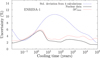 |
Fig. 4 Calculated uncertainties (from nuclear data and total uncertainties) and standard deviation for the 4 decay heat calculations for the segment containing sample ENRESA-1. |
6 Conclusion
In this work, eight BWR samples from the Spanish proprietary experimental program were analyzed in terms of isotopic compositions and decay heat, within the context of the European project EURAD Work Package 8. Different modelization approaches were followed, indicating various degrees of agreement with measured values. For a selection of measured isotopic concentrations, the prediction power indicates a lower level of agreement compared to PWR samples, as also noticed in various publications. This might originate in the complexity of correctly reproducing local (at the assembly level) BWR irradiation history, as well as in the need of precise and thorough description of the irradiation conditions. Calculated uncertainties on isotopic compositions and decay heat indicate the strong impact of nuclear data covariances, and their important changes from one nuclear data library to another. The next most important quantity is the void fraction, affecting a large number of calculated quantities, including 235U and 239Pu concentrations and decay heat. Finally, it was also observed that differences in modeling, not included in the calculated uncertainties, can lead to strong differences, for both the isotopic concentrations and the decay heat.
Conflict of interests
The authors declare that they have no competing interests to report.
Funding
This work was partly supported by swiss nuclear, the association of the Swiss nuclear power station operators, with the COLOSS project. It was also partly funded by the European Union's Horizon 2020 Research and Innovation Programme under grant agreement No 847593 (project EURAD, Work Package 8).
Data availability statement
This article has no associated data generated and/or analyzed.
Author contribution statement
All authors equally contributed to this project.
Appendix A
Uncertainties ΔC from nuclear data libraries for the ENRESA samples for the isotopic concentrations (CASMO5-1 calculations). All values are in %. The last three columns present the maximum uncertainties (due to nuclear data) for the PWR samples GU1, GU3 and BM1 (BM1 being a MOX sample).
Uncertainty intervals ΔC from various parameters for the ENRESA-1 sample for the isotopic concentrations (CASMO5-1 calculations). All values are in %. The contribution from TFU is between 0.0 and 0.1%. The column Sum is the square root of the quadratic sum of the different components.
Expanded estimated uncertainties Δexpanded (based on RSSuc) for isotopic concentrations for the sample ENRESA-1, taking into account the calculation bias and the experimental and calculated uncertainties. ΔCmax come from the nuclear data library leading to the highest nuclear data uncertainty (either ENDF/B-VIII.0, JEFF-3.3 or JENDL-4.0).
Summary of all uncertainties in % (or 1σ) considered in this study for the calculated decay heat at the end of irradiation of the ENRESA-1 sample. The decay heat is indicative and for the position of sample 1. The min – max of the sum (being  for calculated uncertainties) is due to the differences from nuclear data uncertainties.
Expanded estimated uncertainties Δexpanded for the decay heat from the ENRESA-1 sample, taking into account the main calculation biases for isotopic concentrations from Table A.3 and calculated uncertainties from Table A.4. ΔCmax come from the nuclear data library leading to the highest nuclear data uncertainty (either ENDF/B-VIII.0, JEFF-3.3 or JENDL-4.0).
References
- J. Rhodes, K. Smith, D. Lee, CASMO-5 development and applications, in Proceedings of the PHYSOR-2006 conference, ANS Topical Meeting on Reactor Physics, Vancouver, BC, Canada, September 10-14, Vancouver, BC, Canada, September 10-14 (2006), p. B144 [Google Scholar]
- U. Mertyurek, M.W. Francis, I.C. Gauld, SCALE 5 Analysis of BWR Spent Nuclear Fuel Isotopic Compositions for Safety Studies, Oak Ridge National Laboratory Report, ORNL/TM-2010/286 (2010) [Google Scholar]
- D. Rochman, A. Vasiliev, H. Ferroukhi, M. Hursin, Analysis for the ARIANE GU1 sample: nuclide inventory and decay heat, Ann. Nucl. Energy 160, 108359 (2021) [CrossRef] [Google Scholar]
- D. Rochman, A. Vasiliev, H. Ferroukhi, M. Hursin, R. Ichou, J. Taforeau, T. Simeonov, Analysis for the ARIANE GU3 sample: nuclide inventory and decay heat, EPJ Nuclear Sci. Technol. 7, 14 (2021) [CrossRef] [EDP Sciences] [Google Scholar]
- D. Rochman, A. Vasiliev, H. Ferroukhi, M. Hursin, Analysis for the ARIANE BM1 and BM3 samples: nuclide inventory and decay heat, EPJ Nuclear Sci. Technol 7, 18 (2021) [CrossRef] [EDP Sciences] [Google Scholar]
- H.J. Smith, I.C. Gauld, U. Mertyurek, Analysis of Experimental Data for High Burnup BWR Spent Fuel Iso-topic Validation - SVEA-96 and GE14 Assembly Designs, Oak Ridge National Laboratory report NUREg/cR-7162, ORNL/TM-2013/18 (2013) [Google Scholar]
- I.C. Gauld, U. Mertyurek, Validation of BWR spent nuclear fuel isotopic predictions with applications to burnup credit, Nucl. Eng. Des. 345, 110 (2019) [CrossRef] [Google Scholar]
- C. Alejano, J.M. Conde, M. Quecedo, M. Lloret, J.A. Gago, P. Zuloaga, F.J. Fernandez, PWR and BWR Fuel Assay Data Measurements, International Workshop on Advances in Applications of Burnup Credit for Spent Fuel Storage, Transport, Reprocessing and Disposition, Cordoba, Spain (October 2009) [Google Scholar]
- European Joint Programme on Radioactive Waste Management, EU H2020-Euratom-1.2 program, Grant agreement ID: 847593, https://cordis.europa.eu/project/id/847593 [Google Scholar]
- A. Munoz, Specification of measured isotopic concentrations of BWR Spent Fuel, October 26, 2020, ENRESA report INF-TD-010032 Revision 1 [Google Scholar]
- J.M. Conde, C. Alejano, J.M. Rey, Nuclear fuel research activities of the Consejo de Seguridad Nuclear, Top Fuel 2006, International Meeting on LWR fuel Performance Nuclear Fuel: Addressing the Future, 22-26 October 2006 Salamanca, Spain, p. 107, https://euronuclear.info/events/topfuel/transactions/Topfuel-Technical-Session.pdf [Google Scholar]
- I.C. Gauld, U. Mertyurek, Margins for Uncertainty in the Predicted Spent Fuel Isotopic Inventories for BWR Burnup Credit, Oak Ridge National Laboratory report, NUREG/CR-7251 and ORNL/TM-2018/782 (2018) [Google Scholar]
- J.S. Martinez, B.J. Ade, S.M. Bowman, I.C. Gauld, G. Ilas, W.J. Marshall, Impact of modeling choices and inventory and in-cask criticality calculations for Forsmark 3 BWR Spent Fuel, International conference on nuclear criticality safety, ICNC 2015, Charlotte, NC, USA, 13-17 September 2015, p. 14 [Google Scholar]
- D.E. Mueller, S.M. Bowman, W.J. Marshall, J.M. Scaglione, Review and Prioritization of Technical Issues Related to Burnup Credit for BWR Fuel, U.S. Nuclear Regulatory Commission, February 1973, NUREG/CR-7158 and ORNL/TM-2012/261 [Google Scholar]
- E.L. Georgieva, J. Hykes, R.M. Ferrer, J. Rhodes, CASMO5 isotopic comparison to the ARIANE mixed-oxide pressurized water spent fuel measurements, in Proceedings of the PHYSOR 2018 conference: Reactor Physics paving the way towards more efficient systems, Cancun, Mexico, April 22-26, 2018 (2018), p. 1171. [Google Scholar]
- M. Brovchenko, J. Taforeau, Pin power calculation scheme for reactor pressure vessel fast neutron fluence estimation, EPJ Web Confer. 247, 02029 (2021) [CrossRef] [EDP Sciences] [Google Scholar]
- J. Li, D. Rochman, A. Vasiliev, H. Ferroukhi, J. Herrero, A. Pautz, M. Seidl, D. Janin, Bowing effects on isotopic concentrations for simplified PWR assemblies and full cores, Ann. Nucl. Energy 110, 547 (2017) [CrossRef] [Google Scholar]
- D. Rochman, P. Mala, H. Ferroukhi, A. Vasiliev, M. Seidl, D. Janin, J. Li, Bowing effects on power and burn-up distributions for simplified full PWR and BWR cores, in Proceedings of the International Conference on Mathematics and Computational Methods Applied to Nuclear Science and Engineering (M & C), Jeju, Korea, April 16-20, 2017, on USB (2017) [Google Scholar]
- B.T. Bearden, M.A. Jessee, SCALE Code System, ORNL/TM-2005/39 Oak Ridge National Laboratory, Oak Ridge, Tennessee, USA (2018) [Google Scholar]
- A. Shama, D. Rochman, S. Caruso, A. Pautz, Validation of spent nuclear fuel decay heat calculations using Polaris, ORIGEN and CASMO5, Ann. Nucl. Energy 165, 108758 (2022) [CrossRef] [Google Scholar]
- D.A. Brown et al., ENDF/B-VIII.0: The 8th Major Release of the Nuclear Reaction Data Library with CIELO-project Cross Sections, New Standards and Thermal Scattering Data, Nucl. Data Sheets 148, 1 (2018) [CrossRef] [Google Scholar]
- A.J.M. Plompen et al., The joint evaluated fission and fusion nuclear data library, JEFF-3.3, Eur. Phys. J. A 56, 181 (2020) [CrossRef] [Google Scholar]
- K. Shibata et al., JENDL-4.0: a new library for nuclear science and engineering, J. Nucl. Sci. Technol. 48, 1 (2011) [CrossRef] [Google Scholar]
- W. Wieselquist, T. Zhu, A. Vasiliev, H. Ferroukhi, PSI methodologies for nuclear data uncertainty propagation with CASMO-5M and MCNPX: results for OECD/NEA UAM Bench-mark Phase I, Sci. Technol. Nucl. Install. 2013, 549793 (2013) [Google Scholar]
- O. Leray, H. Ferroukhi, M. Hursin, A. Vasiliev, D. Rochman, Methodology for core analyses with nuclear data uncertainty quantification and application to swiss PWR operated cycles, Ann. Nuclear Energy 110, 547 (2017) [CrossRef] [Google Scholar]
- S.D. Phillips, K.R. Eberhardt, B. Parry, Guidelines for expressing the uncertainty of measurement results containing uncorrected bias, J. Res. Natl. Inst. Stand. Technol. 102, 577 (1997) [CrossRef] [Google Scholar]
- D. Rochman, A. Vasiliev, H. Ferroukhi, M. Seidl, J. Basualdo, Improvement of PIE analysis with a full core simulation: the U1 case, Ann. Nucl. Energy 148, 107706 (2020) [CrossRef] [Google Scholar]
- T. Simeonov, CMS5/SNF Validation Isotopic analyses of UOX samples irradiated in BWR Forsmark 3, Studsvik report, SSP-19/402 Revision 0, December 201, Studsvik report, SSP-19/402 Revision 0, December 2018 8 [Google Scholar]
- F. Jatuff, F. Giust, J. Krouthen, S. Helmersson and R. Chawla, Effects of void uncertainties on the void reactivity coefficient and pin power distributions for a 10 x 10 BWR assembly, Ann. Nucl. Energy 33, 119 (2006) [CrossRef] [Google Scholar]
- G. Windecker, H. Anglart, Phase distribution in a BWR fuel assembly and evaluation of a multidimensional multifield model, Nucl. Technol. 134, 49 (2001) [CrossRef] [Google Scholar]
Cite this article as: Dimitri Rochman, Alexander Vasiliev, Hakim Ferroukhi, Ana Muñoz, Miriam Vazquez Antolin, Marta Berrios Torres, Carlos Casado Sanchez, Teodosi Simeonov, and Ahmed Shama. Analysis of ENRESA BWR samples: nuclide inventory and decay heat, EPJ Nuclear Sci. Technol. 8, 9 (2022)
All Tables
Characteristics of the ENRESA samples, as found in the literature and this work (from the CASMO5-1 simulations). The axial height is measured from the bottom of the fuel rod end plug.
Uncertainties ΔC from nuclear data libraries for the ENRESA samples for the isotopic concentrations (CASMO5-1 calculations). All values are in %. The last three columns present the maximum uncertainties (due to nuclear data) for the PWR samples GU1, GU3 and BM1 (BM1 being a MOX sample).
Uncertainty intervals ΔC from various parameters for the ENRESA-1 sample for the isotopic concentrations (CASMO5-1 calculations). All values are in %. The contribution from TFU is between 0.0 and 0.1%. The column Sum is the square root of the quadratic sum of the different components.
Expanded estimated uncertainties Δexpanded (based on RSSuc) for isotopic concentrations for the sample ENRESA-1, taking into account the calculation bias and the experimental and calculated uncertainties. ΔCmax come from the nuclear data library leading to the highest nuclear data uncertainty (either ENDF/B-VIII.0, JEFF-3.3 or JENDL-4.0).
Summary of all uncertainties in % (or 1σ) considered in this study for the calculated decay heat at the end of irradiation of the ENRESA-1 sample. The decay heat is indicative and for the position of sample 1. The min – max of the sum (being for calculated uncertainties) is due to the differences from nuclear data uncertainties.
Expanded estimated uncertainties Δexpanded for the decay heat from the ENRESA-1 sample, taking into account the main calculation biases for isotopic concentrations from Table A.3 and calculated uncertainties from Table A.4. ΔCmax come from the nuclear data library leading to the highest nuclear data uncertainty (either ENDF/B-VIII.0, JEFF-3.3 or JENDL-4.0).
All Figures
|
Fig. 1 Assembly GN592, GE-14 type, with various rod types. The rod J8 containing the 8 samples is indicated in red for the transverse view. On the right is indicated the axial sample positions. Segments in green corresponds to natural uranium [6]. |
| In the text | |
|
Fig. 2 Comparison for calculated and measured nuclide concentrations between the four types of calculations (top: actinides, bottom: fission products). In each subbox, data are ordered from left to right as a function of the sample vertical elevation. |
| In the text | |
|
Fig. 3 Left: calculated decay heat for the segment containing the sample ENRESA-1. Right: calculated decay heat uncertainty for the same segment: comparison with other samples assuming same input uncertainties (top) and contributions to the total uncertainties (bottom). |
| In the text | |
|
Fig. 4 Calculated uncertainties (from nuclear data and total uncertainties) and standard deviation for the 4 decay heat calculations for the segment containing sample ENRESA-1. |
| In the text | |
Current usage metrics show cumulative count of Article Views (full-text article views including HTML views, PDF and ePub downloads, according to the available data) and Abstracts Views on Vision4Press platform.
Data correspond to usage on the plateform after 2015. The current usage metrics is available 48-96 hours after online publication and is updated daily on week days.
Initial download of the metrics may take a while.