| Issue |
EPJ Nuclear Sci. Technol.
Volume 12, 2026
|
|
|---|---|---|
| Article Number | 13 | |
| Number of page(s) | 15 | |
| DOI | https://doi.org/10.1051/epjn/2026005 | |
| Published online | 19 May 2026 | |
https://doi.org/10.1051/epjn/2026005
Regular Article
Bias and uncertainty estimates for in-core LWR reaction rate distributions
Reactor Physics and Thermal hydraulic Laboratory, Paul Scherrer Institut, Villigen, Switzerland
* e-mail: This email address is being protected from spambots. You need JavaScript enabled to view it.
Received:
10
January
2026
Received in final form:
23
March
2026
Accepted:
7
April
2026
Published online: 19 May 2026
Abstract
We analyze in-core reaction rate measurements coming from three Pressurized Water Reactors and two Boiling Water Reactors (named E) and compare them with CASMO5 and SIMULATE-3 (and -5) calculations (named C). A total of almost 1 million experimental values were considered, covering various cycles, detector systems and locations, as well as UO2 and MOX fuel types. Biases and root mean square values (rms) were extracted based on (E − C)/C ratios, leading to the finding of outliers, most likely due to detector issues and possible modeling effects for locations with low power. The average rms value is 2.9%, once the outliers are removed, but dissimilar values are obtained for different reactor types. The effect of nuclear data is also quantified for one PWR, leading to an absolute average rms uncertainty of 0.3%. We conclude, based on this study, that an improvement of the local rms values can be achieved by a better knowledge of measurements (i.e. uncertainties) and a possible update on specific parts of the involved models.
Present address: National Cooperative for the Disposal of Radioactive Waste, Nagra, Wettingen, Switzerland.
© D. Rochman et al., Published by EDP Sciences, 2026
 This is an Open Access article distributed under the terms of the Creative Commons Attribution License (https://creativecommons.org/licenses/by/4.0), which permits unrestricted use, distribution, and reproduction in any medium, provided the original work is properly cited.
1. Introduction
Power distribution measurements are routinely carried out within the cores of commercial light water reactors (LWR). They are performed to satisfy a number of requirements: support of analysis of fuel and cladding integrity, of the reactor control operations, and to evaluate off-line the characteristics of the core. Such measurements directly infer on the compliance with a number of safety criteria, such as not exceeding specific limits for peaking factors or linear heat generation rate, allowing the reactor to be run at its full and optimal conditions [1].
Detector systems used for in-core measurements do not provide a direct measure of the local power distribution, but rather provide reaction rates, for instance based on fission chamber signals (with enriched 235U) or activation methods (with vanadium wires). Therefore the measured quantities need to be corrected for a number of experimental conditions and converted to power for the part of the fuel assembly of interest. Such conversion can be performed with off-line computers, based on “form functions” (also called conversion factors) being dependent on a number of localized plant parameters (fuel burnup, coolant characteristics, control rod locations, etc.) [2, 3].
Once the measured signals are converted into localized power, such “measured power distributions” (such quantity will be referred to in the following as measured power, measured local power, or measured power distribution), as a function of axial and radial locations, can be used to assess how close a core is to safety or operating system settings during normal modes of plant operation. There is therefore a need for uncertainty estimation on such measurements, and similarly for assessing uncertainties coming from the analytical interpretation (based on conversion factors). Such estimations are based on systematic comparisons between such measured power distributions and those purely calculated coming from a core simulator, as presented in the following.
The present type of validation work was performed in the past, for specific plants and dedicated to specific quantities, such as the fuel burnup [3–5]. We are presently proposing to study the difference between measured and calculated local power values (called in the following B = (E − C)/E, E being the measured value and C the calculated one; the ratio is provided in the following in percent) for 5 LWRs, with a total of 977 949 measurements, for different radial and axial positions, different cycles, fuel types, enrichments and burnup values. The term bias will then refer to B, given in percent, eventually described with mean values, standard deviations and root mean squares. For anonymity, the name of these plants will not be disclosed, but a minimum information will be provided. A number of details on the plants, measurements, simulation tools will be given in the following, and results will be presented in terms of distributions of biases, with various quantities such as mean biases (being  and Bi = (Ei − Ci)/Ei, i being a specific case from the measurements) and root mean squares (rms, with rms2 = mean2 + std2 and std: the standard deviation
  ). Other quantities were additionally analyzed, such as median, standard deviations, extreme values, as well as different moments of the distributions, but the following results will focus on the mean and rms for simplicity (except for nuclear data).
Regarding uncertainties, we will focus on calculated uncertainties due to nuclear data (e.g. microscopic cross sections). Experimental uncertainties are unfortunately not provided with the experimental values, and will therefore be left off this work (interested readers are referred for instance to Ref. [4]). A number of studies can be found in the literature for uncertainties due to nuclear data, taking into account full core calculations and realistic LWR cycles. Related to the present study, we can mention reference [6], where the same Boiling Water Reactor (BWR) as one of the cores studied in the following was considered, as well as reference [7] for two similar Pressurized Water Reactors (PWR). In both publications, the impact of the nuclear data on relative fission rates is indicated for specific cases, with uncertainties on rms very similar to the present study, but based on different nuclear data covariance files (ENDF/B-VII.0 and ENDF/B-VII.1). We will show in the following that even if the uncertainties due to nuclear data are expected to be small, they vary within cycles and for different core locations, and can be locally as large as 4% on the local biases (such as the top and bottom of assemblies). The covariance library used here is ENDF/B-VIII.0, and the importance of actinides such as 239Pu will be outlined. For comparison, results of the JEFF-3.3 and JENDL-4.0 nuclear data library covariances are also mentioned.
For the studied cases, the improvement of the agreement between measured and calculated reaction rates most likely necessitates more precise measurements and improved modeling.
2. Studied cases
A total of 977 949 E − C values were analyzed, obtained from a total of 5 LWRs, consisting in 2 BWRs and 3 PWRs. Such values were obtained for different fuel types (UO2 and MOX), various enrichments and core burnup values. For each cycle, core follow calculations were performed with different versions of CASMO5 [8] and SIMULATE (–3 and 5). Details are provided in the following.
2.1. Plants and cycles
As mentioned, data from two BWRs and three PWRs with a number of cycles and assembly information are provided in Table 1. Only for one BWR, named BWR1, data from the first starting reactor cycle are used, whereas for the other ones, the analysis is based on later cycles.
Considered plants, cycles and fuel enrichments (averaged over the active part of the fuel). EFPD corresponds to Effective Full Power Days.
They contained different assembly geometries, with various cases for the BWRs, and a more limited set for the PWRs. More than 75% of PWR cycles contained different numbers of MOX assemblies, and all BWR cycles contained assemblies with burnable absorbers. In more recent cycles, the initial 235U enrichment was increased, and with the use or reprocessed uranium, it can be slightly higher than 5.0% to compensate for the presence of 236U. In total, many different cases were used in the studied cycles, and results will be presented for different groups, when appropriate.
2.2. Measurements
As mentioned in the introduction, in-core measurement systems are used to provide axial and radial neutron flux distribution information within the reactor core. Depending on the reactor type, different measurement systems can be used inside the core: fixed, movable, or both. In this work measurements from the detectors described in Table 2 were analyzed.
Measurement movable system and characteristics for the detector numbers at different locations.
Some general details on these detectors are given in the following, considering two types of measurement systems, being traversing in-core probes and aeroballs:
-
Aeroball system. A movable flux mapping system, or Aeroball system, is based on activation probes, made of a number of steel balls (about 1.7 mm in diameter) and stacked in specific assembly guided tubes. The steel contains a given percentage of vanadium and 51V is activated by neutron capture. When not in use, the ball stacks are kept outside the core. For measurements, all stacks are transported into the active core height with a pneumatic system. The measurement time is about a few minutes, and the ball stacks are then removed. Gamma emitted by the decay of 52V are then detected outside the core. Details can be found in references [4, 9, 10].
-
Traversing in-core probe (TIP). The Traversing In-core Probes, or TIPs, generally consist of multiple independent miniature 235U fission chambers or gamma detectors, inserted when needed in separate axial guide tubes. TIPs can eventually be calibrated with fixed in-core detectors. For the fission chambers, they are often built of titanium, with an internal coating of uranium enriched to over 90% in 235U. The active part of the detector is in the order of 2.5 cm long and 0.5 cm in diameter. For gamma detectors, they often consist in ionization chambers, being made of a metallic cylindrical shell filled with gas.
As indicated in Table 2, such detectors are located at different assembly positions in the cores, and allow to obtain reaction rates for different radial and axial positions. Within one specific cycle, measurements are regularly taken, for instance every 30 days. Two examples are presented in Figure 1 for the PWR3 and BWR2 for given detector positions through a reactor cycle.
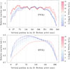 |
Fig. 1. Examples of relative measured reaction rates for the PWR3 and BWR2, at the same radial positions and for various vertical elevation (or axial position), in a specific cycle, for different cycle core burnup. Colors indicate the core burnup values. |
On this figure, one can see the relative measured reaction rates for a specific cycle at one specific radial position for each core. Values for different vertical elevations (or axial positions) are plotted. Colors indicate the total burnup of the considered cores (the value of zero corresponds to the beginning of the cycle, and the highest value corresponds to the end of the cycle). Increasing core burnup is equivalent to increasing cycle time. As observed, for one cycle, about 10 measurement campaigns are taken. Naturally, from one cycle to the next, the assemblies containing the measurement system or next to the TIP detectors are changing due to the assembly shuffling from one cycle to the next, but the locations of the measurements are the same. No uncertainties on the measurements are available for the present study, and related remarks can be found in Section 5.
Such measurements reflect many parameters, such as detector position, the characteristics of the assemblies where the measurements are taken, and the irradiation or cycle histories that the assemblies are experiencing. In order to avoid undesirable effects from the start-up of each cycle on reaction rates, the considered measurements are only for core burnup larger than 0.2 GWd/t. As indicated in Table 2, the total number of considered measurement points is 977 949 in such case.
2.3. Simulation tools
All cycles and all plants were systematically analyzed with the same set of simulation codes, being CASMO5 and SIMULATE-3 or SIMULATE5. Depending on the plant, different versions of these codes were used, as presented in Table 3. In this table and in the following, the abbreviations “sim3” and “sim5” correspond to SIMULATE-3 and SIMULATE5, respectively.
Simulation codes and versions (see text for details). “sim3” refers to SIMULATE-3 and “sim5” to SIMULATE5.
CASMO5 is a lattice physics code for general LWR analysis. All assemblies are modeled with CASMO5, based on fuel vendor characteristics, and complete case matrices are formatted to generate libraries, containing few-group cross sections, reaction rates, discontinuity factors, currents, surface and average fluxes. The nuclear data library used for all calculations is ENDF/B-VII.1 (library version 201, as referenced in CASMO5). Such matrix files are then processed by the utility tool called CMSLINK (or CMSLINK5) to create libraries ready to be used by SIMULATE-3 (or SIMULATE5). SIMULATE is an advanced multi-group nodal code for the analysis of both PWRs and BWRs [11] (in the present case, two-group calculations are performed). The comparison between the calculated and measured three-dimensional in-core reaction rate maps can be easily performed with two post-processing and plotting tools, named S3CORE (for PWR) and S3POST for (BWR). These codes are part of the Studsvik Core Management System (CMS) code package, and are used in this context to compare the measured (E) and calculated (C) reaction rate maps. To illustrate a distribution of the E and C values, Figure 2 is presenting two comparisons as a function of axial nodes, for specific radial measurement positions in the PWR3 and BWR1 cores.
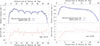 |
Fig. 2. Examples of comparison between the calculated and measured reaction rates (top) and relative difference (bottom), for the PWR3 (left) and BWR1 (right). |
Mean and rms values for the bias distributions, in percent, for all the studied systems. These values are integrated over all cycles. Top: outliers have been removed from the distributions; Bottom: same with outliers included.
In this table, results for both units PWR1 and PWR2 have been combined due to the similarity of the cores and their fuel assemblies. As detailed in the following, the total number of measurements is reduced due to (1) the removal of a number of outliers, mainly detectors presenting bias sensibly different than the other ones (3 detectors for the BWR1 and 2 detectors for BWR2) and (2) (representing the strongest effect) the removal of the bottom and top measurements (details of the analysis are given in the following sections). It can be observed that for the case of PWR3, no measurements were removed, as all bias values were statistically similar. A specific discussion for the identification of outliers is presented in Sections 3.1 and 3.3.
Both measured and calculated relative reaction rates are generally in good agreement, with root mean square values of 2.9% and 0.9% respectively, considering the mean and standard deviation of the 25 or 40 nodes. Note that the vertical scales are different for both core types. Such type of comparison can be done for all radial measurement positions, at different irradiation steps within a cycle, for all cycles, and for the five reactors of interest. Details are in Section 3.
All comparisons presented in the following are obtained with unadjusted core follow models: no model parameters are modified after comparisons between calculated and measured quantities.
2.4. Measurement conversion and comparison
As previously mentioned, the term of “measured reaction rate” is deliberately not precise. The measured quantities are absolute reaction rates, corresponding to a certain position in guide tubes (for PWR) or channels surrounded by fuel bundles (BWR). A number of modifications are necessary in order to obtain derived quantities which can be compared to the calculated ones. The measured signal must first be corrected for signal background, and eventually detector depletion. It must then be converted to a value for the fuel segment of interest. In the case of a PWR, the correction is related to the effect of adjacent vertical segments, and in the case of a BWR, the correction needs to take into account the contributions from different bundles. Other corrections include past assembly exposure, void or boration level, possible control rod movements, and assembly position in the core. Finally, reaction rates are normalized to the total core power and the obtained measured values, called in Figure 2 “derived measurements” can be compared to the calculated relative reaction rates. All such corrections to the measured quantities are automatically performed by the code SIMULATE and the same approach is applied for all the following comparisons.
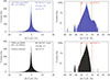 |
Fig. 3. Top: histograms of all (E − C)/E values in %, in linear (left) and logarithmic y-scale (right). Bottom: same, but with outliers removed. |
One can recognize some structures in the plotted data: local minima for the spacer grids for the PWR3, and the low reaction rate values at the bottom and top of the assembly, where the neutron flux is minimal. In the following, results for similar analyses as Figure 2 are presented, for all the measured and calculated values.
3. Bias calculations
In this section, the distributions of the bias (in percent) will be analyzed as a function of many parameters, such as the core type, the detector position, the assembly segment burnup, etc. To summarize the main results of this study, global values are presented in Table 4.
3.1. General observations
The large number of (E − C)/E values, as well as the larger number of detector positions, cycles and fuel assemblies renders the detailed analysis of the results possible only in a statistical way. The most simple approach is to combine all values together, without discrimination. Such distribution is presented in Figure 3 (top) both in linear and logarithmic scales.
It can be observed that the average of all (E − C)/E values is centered on 0.0, with a rms of 3.4%, indicating a good global performance of the simulation scheme. A more detailed observation of the distribution (as presented in logarithmic scale) points to a non symmetric distribution, with a specific structure (or concatenation of values) close to +20%. The tails of the distribution cover a small number of cases, as 99.8% of the histogram counts are within ±20%. Once the outliers have been removed (see Sect. 3.3), as presented in Figure 3 (bottom), the rms is naturally improved, even if the distribution is not symmetric. More details are given in the next sections.
The rule to identify outliers in the following is specific to this study and is not intended to be general. The NIST (National Institute of Standards and Technology) definition of outliers is “An outlier is an observation that lies an abnormal distance from other values in a random sample from a population” [12]. Such definition leaves a certain liberty to decide what is normal and what is abnormal. One example is to declare outliers data points being two or three standard deviations away from the mean of a distribution. In the present case, we are proposing the following definition: for each core unit, a data point being larger than three times the standard deviations is an outlier, such standard deviation being calculated for nodes within the 25th and 75th percentiles (both included). The importance of excluding the bottom and top nodes (which are outside the 25th and 75th percentiles) in this definition will be illustrated in the next section, but it is based on the observation that most of the outliers are not located in the core central part. Such definition of the outliers is not fully statistically justified and other definitions can also be applied. In addition, a physical understanding for the origin of the discrepancies is nevertheless necessary for future improvements, but is not presented in this study.
3.2. BWR and PWR
The first additional analysis of the data is based on the core type, either BWR or PWR. Apart from having different measurement systems, PWR and BWR have different thermalhydraulic processes, fuel types, enrichments and dimensions. It is therefore the first discriminating factor. The mean and rms values for the different distributions are already presented in Table 4. As one can observe, differences appear, indicating smaller rms values for the BWR cores, despite the more complex modeling required to capture their heterogeneities. Mean values are more equally distributed among the cores, and the PWR3 simulations present the largest deviations, on average, compared to measurements. The different histograms are presented in Figure 4. Only values corresponding to SIMULATE-3 are plotted.
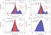 |
Fig. 4. Top: histograms for BWR (E − C)/E values. Bottom: same for PWR values. Calculated values are obtained with SIMULATE-3. |
In the case of both BWR cores, two distinct peaks can be observed, whereas it is not the case for the PWR cores: one centered close to the zero value, and one in the +20 and +30% range. Even if these secondary peaks are of low statistics, they correspond to the same peaks in Figure 3. Additional differentiations will be performed in the next sections to identify the origin of these second peaks. This will give rise of the separation between outliers and standard values.
3.3. Detector positions
The detector position is an important parameter as the rms is known to vary from the center to the periphery of a core. This is expected as the minimum power is reached close to the side of the core, where simulations of the power, reaction rates and other quantities are sensitive to a large number of parameters. For the normal operation of a reactor, larger rms at the side of the core might not be of prime concern, whereas for the back-end management of the fuel cycle, larger rms for assemblies at the reactor side can indicate relevant biases for actinide contents. Figure 5 presents the rms values as a function of vertical position of detectors, also referred to as node.
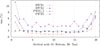 |
Fig. 5. Changes in rms as a function of the detector vertical position (or vertical node). |
For cores with more than 20 nodes, two successive nodes have been averaged in order to reach 20 and to provide a simple comparison (the top and bottom nodes are kept as is, whereas the nodes closer to the center are averaged together). As observed for other reactor cores, the rms distributions globally reach minimum values at the center of the core, whereas higher values are observed at the top and bottom of the core. The tendency can be clearly observed for the PWR1 and 2. Following the outlier definition previously provided, only part of the total E − C values are kept. The two nodes under concern for the PWR1 and 2 are the nodes 1 and 20, and represent about 10% of the data for these two reactor cores. For the BWR1 and 2, the top node 20 is also excluded. The sensitivity to node 20, for both BWRs, is relatively small: if one includes this node in the rms calculations, values given in Table 4 are not significantly modified. On the contrary, rms values are more sensitive to values from each individual detector. Figure 6 presents the rms values for each considered core, as a function of the radial position of the detectors.
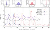 |
Fig. 6. Bottom: same as Figure 5 but a function of the radial position of detectors. Top inserts: the four figures correspond to the labels (1) to (4) given in the bottom figure. |
As the size of the considered cores varies, the number of radial locations also varies: the BWR1 core, being larger than other ones, contains more radial detector locations (the radial detector location is not directly proportional to the distance from the core center). As observed, some rms are relatively constant for different locations (especially for the PWRs), but the BWRs are showing a number of radial positions with sensibly higher rms than other ones: two locations for the BWR2, and three for the BWR1, although one can count four by considering the one at position 24. To represent the impact on the (E − C)/E distributions, four examples are indicated on top of Figure 6, with index numbers from (1) to (4). In the case of locations with higher rms (histograms number (2) and (3)), the (E − C)/E distributions are broader than for cases number (1) and (4), where the rms values are low. The origins of such broad distributions are not yet well understood, possibly originating from wrongly assumed detector vertical locations or inadequate detector modeling. These five radial locations are therefore interpreted as outliers. In conclusion, the following data were considered as outliers and excluded from the final results:
-
for PWR1 and 2, data from the top and bottom nodes (node number 1 and 20 in Fig. 5),
-
for BWR1 and 2, data from the top node (node number 20),
-
for BWR1, data from three radial locations (location 8, 14 and 21 in Fig. 6),
-
for BWR2, data from two radial locations (location 3 and 7).
Removing these outliers has led to the mean and rms values at the top of Table 4, with a reduction of the rms from a global value of 3.4 to 2.9%. As indicated in the tables, not all core values are similar, with a value about 4 times higher for the PWR3 compared to the BWR1 and 2.
3.4. Core cycles and nodal burnup
This section presents the analysis of the rms values as a function of different cycle and assembly quantities. As indicated, no specific feature was observed, and these examples are showing that no outliers could be identified.
The variations of the rms as a function of core cycle are presented in Figure 7. Core cycles are all starting at the index number 1, even if the first analyzed cycle is not the initial reactor cycle. In this case, no particular outstanding rms value for a specific cycle is observed, amid some local tendencies.
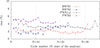 |
Fig. 7. Changes in rms for various selected core cycles. Cycle N is the first analyzed core, different for each reactor. |
Such distributions can also be calculated for each cycle and groups of similar core burnup, to eventually observe a dependence of the mean bias and rms with these quantities. Both quantities were calculated for cycles presented in Table 1, and no significant deviation was observed. Similarly, dividing each cycle in groups of core burnup (e.g. by groups of 5%: from 0 to 5%, up to 95 to 100%) has not indicated differences for the mean and rms values.
Another quantity which can influence the rms is the burnup of the assembly segment where a specific detector is located. In the case of PWR, as the detectors are within a particular assembly, the burnup of the assembly segment is easily identified from the SIMULATE calculation. For BWR cores, as the detector is in between four bundles with each of them having a different segment burnup value, it is less straightforward to extract a representative value. In this case, the average of the four bundle segments is calculated. Results are presented in Figure 8.
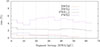 |
Fig. 8. Rms values as a function of the burnup of the assembly segment where the detector is located. |
Once again, no specific pattern, indicating a dependency of the rms with the segment burnup, can be observed. This provides confidence in the simulations of the core cycles and assembly burnup with respect to the measured fission rates.
3.5. Effect of UO2, MOX fuels, and burnable absorbers
As mentioned in Table 1, a number of cycles but not all of the PWRs contained MOX fuels. Consequently, some of the PWR cycles were MOX-free. Based on the variations of the rms in Figure 7, which includes cycles with and without MOX fuel, there is no significant effect. Additionally, the number of MOX assemblies varies from one cycle to the next for a given PWR core. No correlation between the number of MOX assemblies per cycle with the rms value was found. A more detailed study for a specific PWR, separating between detectors within a MOX and UO2 assembly, also indicated no significant difference. We therefore conclude that there is no noticeable effect of the fuel type on the (E − C)/E values.
Similarly for burnable absorbers (BA), specifically considering detectors included in UO2 assemblies with BA, no changes in the (E − C)/E values were observed, compared to cases without BA. We therefore conclude that in the present cases, the various mean and rms values are not sensitive to the presence or absence of burnable absorbers.
4. Impact of nuclear data
4.1. General observations
The uncertainties due to nuclear data can be calculated based on the same models as presented in Table 3. The principle is relatively simple once cycle calculations are automated: repeat n times the same calculations, each time with a different set of nuclear data library. For each of the n calculations, different C values are obtained, reflecting the impact of the different nuclear data libraries. For each calculation with a specific set of nuclear data, SIMULATE is performing a new search of the boron concentration in order to reach a critical core. In total, nE − C values can then be calculated for each detector, leading to probability density functions for which standard deviations (or uncertainties, being defined to one standard deviation) can be extracted. Examples of such method applied to the same reactors are presented in references [6, 13, 14], and the automation scheme is presented in reference [15]. In these references, the focus was not on E − C values for fission rates, but the referenced studies are conveniently supporting the present results.
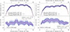 |
Fig. 9. Measured and calculated reaction rates for a specific cycle and detector of the PWR1 (top), and (E − C)/E values (bottom). 70 calculated reaction rates from random nuclear data (all varied at once) are presented. Left: UO2 fuel, Right: MOX fuel. |
In the following, the term nuclear data is limited to microscopic cross sections, number and spectra of emitted particles. The decay data (half-lives, gamma energies, branching ratios) are not included in this work, as it was previously shown that their impact on reaction rates is minor [16]. The uncertainties on nuclear data, or more precisely their covariance matrices are obtained from the ENDF/B-VIII.0 library [17] as the impact of such covariances was of interest. The change of covariance files with respect to the nominal library was already performed for ENDF/B-VII.0 and SCALE-6 covariances in references [6, 7]. In addition, some comparisons with other libraries are also indicated in the following. Perturbation factors in agreement with the covariance matrices are applied to the CASMO5 processed libraries with the in-house tool SHARK-X [16]. All important isotopes are considered (the full list can be found in Ref. [6], Sect. 3): actinides, fission products and structural materials, as well as fission yields. Same variations were used in the previously mentioned references.
One of the drawbacks of such simple method is the required calculation time, virtually multiplying by n the calculation time needed for the results presented in Section 3. For example, one calculation set for BWR1-sim3 is longer than 20 days on a typical CPU, including library generation (CASMO5) and cycle calculations (SIMULATE-3). The calculation of uncertainties was therefore limited to one of the PWR, namely PWR1. A number of different nuclear data were independently sampled and used, in order to assess the effects of individual isotopes:
-
(1)
All nuclear data together. This is performed to assess the total impact of nuclear data, including all relevant actinides and fission products, as well as all fission yields.
-
(2)
Cross sections (and emitted spectra and number of emitted particles) only, for all relevant actinides and fission products.
-
(3)
Fission yields only, for all relevant actinides.
-
(4)
Cross sections (and emitted spectra and number of emitted particles) for 235U only, 238U only, 239Pu only and 241Pu only.
Other isotopes were also individually varied, such as minor actinides (from uranium to curium), light elements (hydrogen and oxygen) and fission products (from Ge to Er), but these results are not detailed here as their effects were minor. For the variations of all nuclear data together (case (1)), n = 330, and for each of the other cases (number (2) to (4)), a total of 100 sampled nuclear data were used, representing a total of more than 800 calculation sets for all cases, with the addition of more than hundreds of calculation sets for other cases not presented due to their small effect. Such value of 100 samples is relatively low, mainly due to the available computer power and the diversity of cases studied. For each of the sampled nuclear data, all cycles are recalculated, implying that a modified specific cross section is used in all cycles of the PWR1. As the quantity of interest is the standard deviation of the calculated (E − C)/E values for a given detector, it can be mentioned that the standard error on the standard deviation varies as  , and with n = 100, the error is about 7% (for n = 330, the error is 4%). Results for the uncertainties on the (E − C)/E values for specific UO2 and MOX assemblies at the middle of cycle are presented in Figure 9.
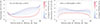 |
Fig. 10. Examples of uncertainties on (E − C)/E due to (all) nuclear data for two different assemblies during a specific PWR cycle. Colors indicate the cycle burnup. |
One can see the effect of (all) nuclear data on the individual reaction rates and (E − C)/E values. In the UO2 specific case (but same observations hold for the MOX case), the average (E − C)/E value (averaged over all segments and all 330 calculations) is –1.5%, with a standard deviation of 1.4% (the nominal calculation, red line in the figure, has an average value of –1.6%). The blue band in the bottom of the figure indicates the standard deviations for each segment. The value of 1.4% reflects the effect of the nuclear data impact, and in this presented case, all nuclear data are varied together. In the following, only the uncertainty (being equal to the standard deviation) on the (E − C)/E values will be presented for simplicity.
4.2. Nuclear data uncertainties as a function of the cycle burnup
The previous examples were given for a specific cycle burnup value (for instance at two thirds of the cycle length), corresponding to an average assembly burnup as indicated in Figure 9. Similar studies can be performed for different cycle burnup values, only focusing on the uncertainty for the (E − C)/E values. Uncertainties due to all nuclear data can be changing depending on the fuel content (i.e. the assembly burnup and the assembly fuel type), and examples for two different cases are presented in Figure 10: a UO2 assembly with different burnup values, and a different MOX assembly, also with different burnup values.
The color scales in this figure refer to the core burnup for the cycle of interest; when increasing, the burnup of the considered assembly is also increasing. As observed in all cases, there is a strong dependence on the axial nodes, as well as on the core burnup. Uncertainties tend to be lower for higher burnup values, with an inverse shape between UO2 and MOX assemblies as a function of nodes. The range of uncertainty is globally between 0.5 and 5%, overlapping with values from references [6, 13, 14], but also showing a more detailed pattern. These two examples may be not representative to all UO2 or MOX assemblies with different burnup values, as the uncertainties may also depend on the enrichment of the considered assembly at the beginning of cycle. In the present case, as shown in the figure, two burnup values are considered (one for the UO2 assembly and one for the MOX assembly), and other assemblies can have different burnup values.
In addition to these estimations based on the ENDF/B-VIII.0 covariance data, the nuclear data library covariance files from the JEFF-3.3 and JENDL-4.0 were used [18, 19]. In both cases, similar shapes and dependencies were found as the ones presented in Figure 10, but the amplitude of the uncertainties were lower, reaching maximum values of 2 (JEFF-3.3) and 2.5% (JENDL-4.0) for the UO2 case and 2% for the MOX case.
To understand part of the origin of the uncertainty amplitudes and shapes, partial variations of nuclear data were used, as previously explained, such as nuclear data related to specific actinides only (e.g.235U), all fission products together, or only fission yields. The main contributors to the total effects are presented in Figure 11 for the cases with the highest burnup indicated in Figure 10.
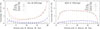 |
Fig. 11. Decomposition of the nuclear data uncertainties for two UO2 and MOX assemblies based on the ENDF/B-VIII.0 covariance files. |
It is interesting to note that in all cases, the 239Pu nuclear data are the main source of uncertainties. 239Pu can be present in the assembly where the detector is located, if such assembly is of MOX type, or if it is of UO2 type with high enough burnup. It is also present in other assemblies, as the cycle of interest is considered at equilibrium. The observed effect is therefore both local (possible 239Pu contained in the assembly of interest) and global (from 239Pu contained in other assemblies and still affecting the core neutronic characteristics). The reason for the inverse shape of uncertainties between MOX and UO2 fuel types is not yet understood, apart from the fact that less 239Pu is generally contained in the top and bottom segments (due to low burnup values). Additional work dedicated to this effect would be necessary. In addition, the study of the first reactor cycle would be of interest, as all fuel assemblies are fresh and 239Pu is not present in the core.
The same analysis was performed with the JEFF-3.3 and JENDL-4.0 covariance matrices, and similar conclusions hold, with the difference that the effect of 239Pu is lower for both libraries, nevertheless staying the main source of uncertainties.
4.3. Comparison with biases for the PWR1
As a final remark, the uncertainties presented in the three last figures were given for the (E − C)/E values, as one standard deviation. They come strictly from variations of the calculated reaction rates C, and are not affected by the measured values E. One of the goals of this study is eventually to compare biases and uncertainties, and as biases were presented with the rms quantities, it is also useful to express the impact of nuclear data in terms of rms. Additionally, due to the limitation in computer power, only six consecutive equilibrium cycles of the PWR1 were considered for the uncertainty propagation. For each of the random sampling performed for all nuclear data (300 cases for the ENDF/B-VIII.0 library, and 100 for the two other ones), the individual mean (E − C)/E and rms values for the six cycles of interest were calculated and are presented in Table 5.
Top line: nominal mean and rms (in %) for (E − C)/E, considering 6 PWR1 cycles (no nuclear data variation). Other lines: standard deviations for the mean and rms due to the variation of all nuclear data, based on three different nuclear data covariance sets.
The nominal cases (without nuclear data variations) correspond to values presented in Section 3. The other values were obtained by varying nuclear data, and standard deviations on the mean and on the rms are presented. For instance, in the case of Cycle 1 and the ENDF/B-VIII.0 covariance library, the 300 rms values (one for each of the 300 realizations of the nuclear data sampling) have a standard deviation presented in the table with the label σmean. Similarly, the width of the rms distribution can be quantified with a standard deviation, provided in the table with σrms. These quantities are calculated using the covariance matrices for the three libraries listed in the table, and the six cycles named 1 to 6. To illustrate the distribution of the calculated rms and mean values based on covariance data, Figure 12 presents the case of the cycle 2 and the ENDF/B-VIII.0 library.
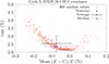 |
Fig. 12. Example for the Cycle 2 and the ENDF/B-VIII.0 covariance with the 300 calculated mean (E − C)/E and rms. Note that the distribution is strongly skewed. The uncertainties on the average correspond to the standard deviation, while for the median, the median average deviation (or MAD) is used. |
As observed, a large range of mean and rms values are obtained with the 300 random set of nuclear data. Due to the non normality of the distribution, the median is different from the average, and the standard deviation also deviates from the median average deviation (both are presented in the figure). Only the standard deviations are presented in Table 5, but other quantifiers (average and median, together with the standard deviations and median average deviations) can be used to represent the impact of nuclear data.
For a specific cycle, the changes of the rms can be more important for larger rms values (i.e as presented by the parabolic shape of the curve) and indicated that the nominal libraries are already performing relatively well. A more pronounced gain for the mean (E − C)/E can be observed (larger spread on the x axis than on the y axis). A reduction of rms, if any, should be assessed over a wide range of cycles, as it was observed that the gain for the presented cycles (with a specific random nuclear data library) does not automatically lead to a gain for another cycle. It was observed that two successive cycles might be highly correlated (with a correlation value higher than 0.90), but such correlation rapidly decreases between cycles separated by one of more cycles. A detailed study can be performed, for instance as a function of cycles, detector position or core burnup, given a higher number of cycles for which the nuclear data impact is evaluated.
Compared to the rms distributions from reference [7] (Fig. 14 in this reference), the uncertainty (or standard deviation) on the reported rms values are very similar to the values for Table 5: the changes of amplitudes agree between both studies, even if the considered covariance matrices are different.
5. Discussion
The present study was divided in two complementary parts: the comparison of the calculated and measured in-core reaction (fission) rates and the impact of nuclear data on the calculated fission rates. The comparison of the E and C quantities is part of the validation of the various CASMO5 and SIMULATE models, and if such work would be simplified to a single number, the rms of all (E − C)/E values is 2.9% (see Tab. 4, with dissimilar values for different reactor types). In comparison, the impact of nuclear data on the rms is about (2.9 ±0.3)% (the value 0.3 represents the average one standard deviation, in the case of the PWR1).
One of the main questions is, can (shall) we still improve the agreement between calculated and measured fission rates, and if yes, what is the best way of doing it. An average rms value of 2.9% might seem low, and is certainly acceptable, or very good, for many applications (such as in-core fuel management and issues related to the safety of the reactor core under normal operation), and it is comparable to values presented in the literature, as in references [20, 21]. From the perspective of the characterization of the spent nuclear fuel, larger rms for core nodes with low burnup values (therefore containing larger amount of fissioning actinides) might lead to significant penalty factors. It is therefore of interest to dedicate efforts to lower the biases and rms values.
Given the impact of nuclear data on rms values, it is not apparent that better nuclear data would lead to strong reduction of rms values.
Regarding improved modeling, it was observed that large discrepancies were obtained for bottom and top segments, as indicated in Figure 5. Even if power and fission reaction rates are low in these locations, it is assumed that the reflector modeling can impact biases (as also shown in Ref. [21]). Improved modeling can certainly help to reduce biases, implying careful studies of each reactor core under consideration, in combination with the characteristics of the simulation code.
Related to the improvement of detector modeling and the accuracy of the measurements, the experimental uncertainty needs to be taken into account in the estimation of the biases. Taking into account experimental uncertainty will lead to probabilistic acceptance of differences between E and C, contrary to the present work where such uncertainty was ignored. The main reason for not taking into account experimental uncertainties is that they are currently not reported with the measured values. The information in the open literature is also scarce. As an example, in reference [21], it is indicated that “the total error of the aeroball measurements amounts to about 1%”. Taking into account 1% experimental uncertainty would modify our understanding of the bias, indicating that an important factor to improve rms values is in fact the experimental uncertainty.
Apart from better modeling and the account for experimental uncertainties, a third aspect to consider for the analysis of biases concerns the uncertainties from models and irradiation assumptions. As for nuclear data, one can for instance propagate the uncertainties due to fuel temperature, moderator density or fuel enrichment. Just as for the experimental uncertainties, they would provide a different perspective on biases.
Finally, the understanding of the biases related to in-core reaction rates can be used to estimate the uncertainties on other quantities such as the assembly burnup. Assembly and pin burnup values are of high importance for safeguards and for the backend of the fuel management (e.g. for decay heat and cask or canister criticality). These quantities are often provided without uncertainties. In the vast majority of cases, assembly or pin burnup values are nevertheless estimated from the core simulator (such as SIMULATE) with a number of assumptions, and in-core reaction rates can be used to estimate assembly burnup or reactivity uncertainties as proposed in references [22, 23]. This task will be presented in a follow study for the same reactors as studied here.
6. Conclusion
In this work, biases between measured (E) and calculated (C) in-core reaction rates were analyzed for five LWRs, based on almost one million values spanning over many reactor cycles. Both MOX and UO2 fuel types were in use, with initial enrichments from 0.8% to 5%. Detector systems were both TIPs and aeroballs, whereas the calculated values were obtained with SIMULATE (version 3 and 5). A number of outliers were identified, and it was found that the mean (E − C)/E was –0.13% with a global rms value of 2.9%. These values may appear very satisfactory, but differences between reactors can be seen in Table 4 and in Figure 4. The analysis was also performed as a function of considered reactor cores, cycles, detector positions and fuel types. The effects of nuclear data were quantified, moderately affecting the rms value by 2.9 with an average standard deviation of ±0.3%. It is proposed that further improvements for biases are achieved by better modeling (reflectors and regions of low power), by estimating the influence of simulation parameters, as well as by considering experimental and modeling uncertainties. The present work can be considered as one of the steps towards more elaborated safety assessment.
Funding
This research did not receive any specific funding.
Conflicts of interest
The authors declare that they have no competing interests to report.
Data availability statement
The data used for this study are not public and are owned by PSI and the power plants.
Author contribution statement
All authors equally contributed to the data analysis and the writing of the present paper.
Acknowledgments
This work was partly funded by the Swiss Nuclear Safety Inspectorate ENSI (H-101230) and was conducted within the framework of the STARS program. We thank Jiri Ulrich from ENSI, for his assistance and dedicated time in reading various drafts of the present paper and in guiding us for adequate formulations.
References
- J.R. Fisher, Review of in-core power distribution measurements, technical status and problems, Tech. Rep. EPRI NP-337, Electric Power Research Institute (EPRI), January 1977. [Google Scholar]
- K. Andrzejewski, Power distribution unfolding on the basis of in-core rhodium powered detector readings, Tech. Rep. IAEA-R-4222-F, International Atomic Energy Agency, October 1988. [Google Scholar]
- J.M. Yedidia, Determination of the accuracy of utility spent fuel burnup records; interim report, Tech. Rep. EPRI TR-109929, Electric Power Research Institute (EPRI), May 1998. [Google Scholar]
- J. Konheiser, M. Seidl, C. Brachem, S. Mueller, Study of the uncertainties due to position change of the PWR aeroball measurement system, J. Nucl. Sci. Technol. 53, 1715 (2016), https://doi.org/10.1080/00223131.2016.1151840 [Google Scholar]
- M. Seidl, P. Schillebeeckx, D. Rochman, Note on the potential to increase the accuracy of source term calculations for spent nuclear fuel, Front. Energy Res. 11, 1143312 (2023), https://www.frontiersin.org/articles/10.3389/fenrg.2023.1143312 [Google Scholar]
- D. Rochman, A. Dokhane, A. Vasiliev, H. Ferroukhi, M. Hursin, Nuclear data uncertainties for core parameters based on Swiss BWR operated cycles, Ann. Nucl. Energy 148, 107727 (2020), https://doi.org/10.1016/j.anucene.2020.107727, https://www.sciencedirect.com/science/article/pii/S0306454920304254 [CrossRef] [Google Scholar]
- O. Leray, H. Ferroukhi, M. Hursin, A. Vasiliev, D. Rochman, Methodology for core analyses with nuclear data uncertainty quantification and application to Swiss PWR operated cycles, Ann. Nucl. Energy 110, 547 (2017), https://doi.org/10.1016/j.anucene.2017.07.006, https://www.sciencedirect.com/science/article/pii/S0306454916311288 [CrossRef] [Google Scholar]
- R.M. Ferrer, J.D. Rhodes, Extension of Linear Source MOC Methodology to Anisotropic Scattering in CASMO5, in International Conference on Physics of Reactors (PHYSOR 2014), September 28-October 3, 2014, Kyoto, Japan, No. JAEA-Conf 2014-003 (2014), https://jopss.jaea.go.jp/search/servlet/search?5049377 [Google Scholar]
- I. Endrizzi, M. Beczkowiak, G. Meier, Refinement of Siemens core monitoring based on aeroball and PDD in-core measuring systems using powertrax, in Workshop proceedings Core monitoring for commercial reactors: improvements in systems and methods, Organisation for Economic Co-Operation and Development, Stockholm (Sweden), 4-5 October, 1999 (1999). [Google Scholar]
- C. Düweke, N. Thillosen, J. Ziethe, Neutron flux incore instrumentation of AREVA’s EPR, in 2009 1st International Conference on Advancements in Nuclear Instrumentation, Measurement Methods and their Applications (2009), pp. 1–6, https://doi.org/10.1109/ANIMMA.2009.5503769 [Google Scholar]
- T. Bahadir, S.O. Lindhal, Studsvik’s next generation nodal code SIMULATE-5, in, Advances in Nuclear Fuel Management IV (ANFM 2009), Hilton Head Island, South Carolina, USA, April 12-15, 2009 (2009). [Google Scholar]
- National institute of Standards and Technology (NIST), NIST/SEMATECH e-Handbook of Statistical Methods, 2012, https://doi.org/10.18434/M32189, http://www.itl.nist.gov/div898/handbook/ [Google Scholar]
- D. Rochman, A. Vasiliev, A. Dokhane, H. Ferroukhi, M. Hursin, Nuclear data uncertainties for Swiss BWR spent nuclear fuel characteristics, Eur. Phys. J. Plus 135, 233 (2020), https://link.springer.com/article/10.1140/epjp/s13360-020-00258-2 [CrossRef] [Google Scholar]
- D. Rochman, A. Vasiliev, A. Dokhane, H. Ferroukhi, Uncertainties for Swiss LWR spent nuclear fuels due to nuclear data, EPJ Nuclear Sci. Technol. 4, 6 (2018), https://doi.org/10.1051/epjn/2018005 [CrossRef] [EDP Sciences] [Google Scholar]
- D. Rochman, A. Vasiliev, H. Ferroukhi, M. Pecchia, Consistent criticality and radiation studies of Swiss spent nuclear fuel: The CS2M approach, J. Hazardous Mater. 357, 384 (2018), https://doi.org/10.1016/j.jhazmat.2018.05.041, https://www.sciencedirect.com/science/article/pii/S0304389418303959 [Google Scholar]
- O. Leray, P. Grimm, M. Hursin, H. Ferroukhi, A. Pautz, Uncertainty quantification of spent fuel nuclide compositions due to cross-sections, decay constants and fission yields, in International Conference on Physics of Reactors (PHYSOR 2014), September 28-October 3, 2014, Kyoto, Japan, No. JAEA-Conf 2014-003 (2014), URL https://jopss.jaea.go.jp/search/servlet/search?5049377 [Google Scholar]
- D.A. Brown, M.B. Chadwick, R. Capote, A.C. Kahler, A. Trkov, M.W. Herman, A.A. Sonzogni, Y. Danon, A.D. Carlson, M. Dunn, D.L. Smith, G.M. Hale, G. Arbanas, R. Arcilla, C.R. Bates, B. Beck, B. Becker, F. Brown, R.J. Casperson, J. Conlin, D.E. Cullen, M.A. Descalle, R. Firestone, T. Gaines, K.H. Guber, A.I. Hawari, J. Holmes, T.D. Johnson, T. Kawano, B.C. Kiedrowski, A.J. Koning, S. Kopecky, L. Leal, J.P. Lestone, C. Lubitz, J.I. Màrquez Damiàn, C.M. Mattoon, E.A. McCutchan, S. Mughabghab, P. Navratil, D. Neudecker, G.P.A. Nobre, G. Noguere, M. Paris, M.T. Pigni, A.J. Plompen, B. Pritychenko, V.G. Pronyaev, D. Roubtsov, D. Rochman, P. Romano, P. Schillebeeckx, S. Simakov, M. Sin, I. Sirakov, B. Sleaford, V. Sobes, E.S. Soukhovitskii, I. Stetcu, P. Talou, I. Thompson, S. van der Marck, L. Welser-Sherrill, D. Wiarda, M. White, J.L. Wormald, R.Q. Wright, M. Zerkle, G. Žerovnik, Y. Zhu, ENDF/B-VIII.0: The 8th Major Release of the Nuclear Reaction Data Library with CIELO-project Cross Sections, New Standards and Thermal Scattering Data, Nucl. Data Sheets 148, 1 (2018), https://doi.org/10.1016/j.nds.2018.02.001, https://www.sciencedirect.com/science/article/pii/S0090375218300206 [CrossRef] [Google Scholar]
- A.J.M. Plompen, O. Cabellos, C. De Saint Jean, M. Fleming, A. Algora, M. Angelone, P. Archier, E. Bauge, O. Bersillon, A. Blokhin, F. Cantargi, A. Chebboubi, C. Diez, H. Duarte, E. Dupont, J. Dyrda, B. Erasmus, L. Fiorito, U. Fischer, D. Flammini, D. Foligno, M.R. Gilbert, J.R. Granada, W. Haeck, F.J. Hambsch, P. Helgesson, S. Hilaire, I. Hill, M. Hursin, R. Ichou, R. Jacqmin, B. Jansky, C. Jouanne, M.A. Kellett, D.H. Kim, H.I. Kim, I. Kodeli, A.J. Koning, A.Y. Konobeyev, S. Kopecky, B. Kos, A. Krása, L.C. Leal, N. Leclaire, P. Leconte, Y.O. Lee, H. Leeb, O. Litaize, M. Majerle, J.I. Márquez Damián, F. Michel-Sendis, R.W. Mills, B. Morillon, G. Noguère, M. Pecchia, S. Pelloni, P. Pereslavtsev, R.J. Perry, D. Rochman, A. Röhrmoser, P. Romain, P. Romojaro, D. Roubtsov, P. Sauvan, P. Schillebeeckx, K.H. Schmidt, O. Serot, S. Simakov, I. Sirakov, H. Sjöstrand, A. Stankovskiy, J.C. Sublet, P. Tamagno, A. Trkov, S. van der Marck, F. Álvarez-Velarde, R. Villari, T.C. Ware, K. Yokoyama, G. Žerovnik, The joint evaluated fission and fusion nuclear data library, JEFF-3.3, Eur. Phys. J. A 56, 181 (2020), https://doi.org/10.1140/epja/s10050-020-00141-9 [CrossRef] [Google Scholar]
- K. Shibata, O. Iwamoto, T. Nakagawa, N. Iwamoto, A. Ichihara, S. Kunieda, S. Chiba, K. Furutaka, N. Otuka, T. Ohsawa, T. Murata, H. Matsunobu, A. Zukeran, S. Kamada, J.I. Katakura, JENDL-4.0: A New Library for Nuclear Science and Engineering, J. Nucl. Sci. Technol. 48, 1 (2011), https://doi.org/10.1080/18811248.2011.9711675 [CrossRef] [Google Scholar]
- A. DiGiovine, A. Noël, GARDEL-PWR: Studsvik’s Online Monitoring and Reactivity Management System, Advances in Nuclear Fuel Management III (ANFM 2003), Hilton Head Island, South Carolina, USA, October 5-8, 2003, on CD-ROM, (American Nuclear Society, LaGrange Park, IL, 2003). [Google Scholar]
- Nuclear Energy Agency (Ed.), Proceedings of a Specialists’ Meeting, Calculation of 3-dimenstional rating distributions in operating reactors (Nuclear Energy Agency, Paris, France, 1979), https://www.oecd-nea.org/upload/docs/application/pdf/2019-12/nea1828-3d79.pdf [Google Scholar]
- K.S. Smith, S. Tarves, T. Bahadir, R. Ferrer, Benchmarks for Quantifying Fuel Reactivity Depletion Uncertainty, Tech. Rep. 1022909, EPRI, Palo Alto, USA, August 2011. [Google Scholar]
- S. Tarves, T. Bahadir, R. Ferrer, Benchmarks for Quantifying Fuel Reactivity Depletion Uncertainty – Revision 1, Tech. Rep. 3002010613, EPRI, Palo Alto, USA, October 2017. [Google Scholar]
Cite this article as: Dimitri A. Rochman, Alexander Vasiliev, Hakim Ferroukhi, Louis Berry, Bias and uncertainty estimates for in-core LWR reaction rate distributions, EPJ Nuclear Sci. Technol. 12, 13 (2026), https://doi.org/10.1051/epjn/2026005
All Tables
Considered plants, cycles and fuel enrichments (averaged over the active part of the fuel). EFPD corresponds to Effective Full Power Days.
Measurement movable system and characteristics for the detector numbers at different locations.
Simulation codes and versions (see text for details). “sim3” refers to SIMULATE-3 and “sim5” to SIMULATE5.
Mean and rms values for the bias distributions, in percent, for all the studied systems. These values are integrated over all cycles. Top: outliers have been removed from the distributions; Bottom: same with outliers included.
Top line: nominal mean and rms (in %) for (E − C)/E, considering 6 PWR1 cycles (no nuclear data variation). Other lines: standard deviations for the mean and rms due to the variation of all nuclear data, based on three different nuclear data covariance sets.
All Figures
|
Fig. 1. Examples of relative measured reaction rates for the PWR3 and BWR2, at the same radial positions and for various vertical elevation (or axial position), in a specific cycle, for different cycle core burnup. Colors indicate the core burnup values. |
| In the text | |
|
Fig. 2. Examples of comparison between the calculated and measured reaction rates (top) and relative difference (bottom), for the PWR3 (left) and BWR1 (right). |
| In the text | |
|
Fig. 3. Top: histograms of all (E − C)/E values in %, in linear (left) and logarithmic y-scale (right). Bottom: same, but with outliers removed. |
| In the text | |
|
Fig. 4. Top: histograms for BWR (E − C)/E values. Bottom: same for PWR values. Calculated values are obtained with SIMULATE-3. |
| In the text | |
|
Fig. 5. Changes in rms as a function of the detector vertical position (or vertical node). |
| In the text | |
|
Fig. 6. Bottom: same as Figure 5 but a function of the radial position of detectors. Top inserts: the four figures correspond to the labels (1) to (4) given in the bottom figure. |
| In the text | |
|
Fig. 7. Changes in rms for various selected core cycles. Cycle N is the first analyzed core, different for each reactor. |
| In the text | |
|
Fig. 8. Rms values as a function of the burnup of the assembly segment where the detector is located. |
| In the text | |
|
Fig. 9. Measured and calculated reaction rates for a specific cycle and detector of the PWR1 (top), and (E − C)/E values (bottom). 70 calculated reaction rates from random nuclear data (all varied at once) are presented. Left: UO2 fuel, Right: MOX fuel. |
| In the text | |
|
Fig. 10. Examples of uncertainties on (E − C)/E due to (all) nuclear data for two different assemblies during a specific PWR cycle. Colors indicate the cycle burnup. |
| In the text | |
|
Fig. 11. Decomposition of the nuclear data uncertainties for two UO2 and MOX assemblies based on the ENDF/B-VIII.0 covariance files. |
| In the text | |
|
Fig. 12. Example for the Cycle 2 and the ENDF/B-VIII.0 covariance with the 300 calculated mean (E − C)/E and rms. Note that the distribution is strongly skewed. The uncertainties on the average correspond to the standard deviation, while for the median, the median average deviation (or MAD) is used. |
| In the text | |
Current usage metrics show cumulative count of Article Views (full-text article views including HTML views, PDF and ePub downloads, according to the available data) and Abstracts Views on Vision4Press platform.
Data correspond to usage on the plateform after 2015. The current usage metrics is available 48-96 hours after online publication and is updated daily on week days.
Initial download of the metrics may take a while.