| Issue |
EPJ Nuclear Sci. Technol.
Volume 12, 2026
|
|
|---|---|---|
| Article Number | 10 | |
| Number of page(s) | 23 | |
| DOI | https://doi.org/10.1051/epjn/2026003 | |
| Published online | 03 April 2026 | |
https://doi.org/10.1051/epjn/2026003
Regular Article
Numerical assessment of spacer grid geometry on turbulence anisotropy in a rod bundle
CEA, DES, IRESNE, Nuclear Technology Department, Centre of Cadarache, Saint-Paul-Lez-Durance F-13108, France
* e-mail: This email address is being protected from spambots. You need JavaScript enabled to view it.
Received:
9
September
2025
Received in final form:
12
December
2025
Accepted:
23
February
2026
Published online: 3 April 2026
Abstract
The highly turbulent flow circulating between the rods inside a Pressurised Water Reactor (PWR) core creates turbulence induced vibrations. To get a better understanding of the flow characteristics, the French Alternative and Atomic Energy Commission (CEA) had built and operated CALIFS 5x5-test section. This mock up composed of a 5-by-5 rod bundle allowed velocity measurements using laser imaging techniques downstream an analytical spacer grid with and without mixing vanes. The CALIFS experiments and other experiments, revealed turbulence anisotropy downstream of spacer grids. The current study aims to assess the impact of spacer grid geometry on the turbulence anisotropy in a rod bundle using fine scale CFD simulation. The study focuses on the characterisation of the anisotropic behaviour of the flow in a rod bundle downstream simplified mixing grids inspired from the CALIFS 5x5 design. Wall-Resolved Large Eddy Simulations (WRLES) are used at a reduced Reynolds number of 14 000. The computation domain is limited to four subchannels around a central rod. Two simulations are performed, using different spacer grids designs (with and without mixing vanes). The results confirm mixing grid design strongly influences the overall turbulence anisotropy. In the case without mixing vanes, the impact of the grid on turbulence anisotropy seems to vanish 10 Hydraulic diameter (Dh) downstream of the grid. In the case with mixing vanes, the anisotropy remains in the subchannels up to 15 Dh downstream of the grid. In both cases, the turbulence anisotropy in the rod vicinity is strongly impacted close to the grid.
© H. Charton et al., Published by EDP Sciences, 2026
 This is an Open Access article distributed under the terms of the Creative Commons Attribution License (https://creativecommons.org/licenses/by/4.0), which permits unrestricted use, distribution, and reproduction in any medium, provided the original work is properly cited.
1. Introduction
Spacer grids with mixing vanes enhance the turbulence intensity in Pressurised Water Reactor (PWR) fuel assemblies. This has the advantage of improving the heat transfer from the rods to the water but it also creates flow induced vibrations which can lead to grid-to-rod fretting. For this reason, the turbulent flows inside PWR have been thoroughly studied using experimental test sections as well as CFD calculations [1].
To this end, the International Atomic Energy Agency (IAEA) has organised the Matis-H benchmark based on the experimental results of the Korean Atomic Energy Research Institute (KAERI). The experimental set up was a horizontal 5x5 rod bundle with two different types of mixing vanes spacer grids. The velocity downstream of a grid was measured by Laser Doppler Anemometry (LDA) at three different locations: 0.5 Hydraulic Diameter (Dh), 4 Dh and 10 Dh downstream of the spacer grid. The two types of vanes were called “split type” and “swirl type”. The Reynolds number of the flow was 50 000. Elliptical eddies generating a cross-flow in the gaps between the rods were observed with the “split type” vanes. With the “swirl” type vanes only circular eddies were observed [2]. At the end of the experiments, the measured velocity fields were shared publicly to organise the CFD benchmark which brought together numerous contributions from several research teams around the globe [3]. The Matis-H benchmark displayed several RANS and URANS simulations using Linear Eddy Viscosity Models such as k-ϵ models and k-ω models [4–9] but also Reynolds Stress Modelling [4–6, 8–10]. These calculations proved to be efficient at estimating consistent averaged velocity field with a correct degree of accuracy. However, RANS calculations remain limited, as they offer only modelled velocity fluctuations. Hence, it is necessary to use high accuracy CFD simulations such as Large Eddy Simulation (LES) that can resolve a large portion of the turbulent spectrum when a precise analysis of turbulent quantities such as the Root Mean Square (RMS) of velocity fluctuations or the Reynolds stresses is required. Such simulations were also performed for the Matis-H benchmark using wall modelled LES [11] or hybrid RANS/LES [12, 13] and gave high quality results despite some discrepancies between the measured and the simulated velocity fluctuations.
The French Alternative and Atomic Energy Commission (CEA) also built several experimental set-ups to study fuel assembly hydro-mechanics [14]. Among these, CALIFS 5x5 is a vertical 5x5 rod bundle with mixing vanes spacer grids. The rods are held in the grid by springs and dimples. The particularity with this test section is that a pressure fluctuations measurement system is put in the central rod. This system allows to measure the pressure and the pressure fluctuations at different angles around the rod wall. Velocity field measurements were also carried out on the test section with Particle Image Velocimetry (PIV) and LDA [15–17]. The LDA results were used to validate a CFD benchmark at Re = 66 000 [18]. Three wall modelled LES have been performed using different software and different sub-grid scale models. Like in the Matis-H benchmark, the three LES gave high accuracy results when predicting the averaged velocity field and the velocity fluctuations. However, some disparities between the evaluations of the pressure fluctuations and the experimental results far away downstream of the grid were observed [18].
One of the possible explanations for the slight discrepancies observed in the benchmark might be the flow anisotropy. When a flow is anisotropic at the largest scales of turbulence, this anisotropy can propagate into smaller scales [19]. Then, when performing a LES to simulate an entire experimental apparatus such as a 5x5 rod bundle, the geometry is often too big to create a mesh sufficiently refined to capture this anisotropy. Moreover, experimental measurements using PIV at Re = 14 000 showed that the flow inside a rod bundle downstream of the mixing vanes of a spacer grid is strongly anisotropic [20]. This observation was made also in the vicinity of the rods, using PIV at Reynolds numbers between 800 and 17 600 [21]. In their study, the team observed that a mixing grid induces the presence of velocity fluctuations in more than one direction of the flow in the viscous sub layer with y + < 5.
With the use of CFD computations, one can have access to the 3 components of the velocity field in every cell of the mesh. This data allows the user to characterise turbulence anisotropy. Using Direct Numerical Simulation (DNS), the anisotropic behaviour of the flow inside a 5x5 rod bundle at Re = 17 600 without mixing grids was characterised [22]. The researchers performed the simulation with Nek5000 and calculated the eigenvalues from the anisotropic part of the Reynolds stress tensor. These eigenvalues were then used to create a colour map based on the idea of other researchers [23, 24]. This map displays the turbulent anisotropy in an entire horizontal plane of the section. The map shows that one component of the velocity fluctuations is far stronger than the two others near the rod wall, and also that the velocity fluctuations tend to become equal while departing from the rods. As a result, the flow tends to become isotropic within the subchannels and gaps. The same process was applied to study the impact of a control rod [25]. Using Wall Resolved LES, it was observed that the presence of a thimble tube can modify this anisotropic behaviour in the gaps between rods.
With the anisotropy having been observed experimentally downstream of a spacer grid the aim of this study is to characterise it using CFD at different locations downstream of the grid, employing the same method as applied to the DNS results [22], in order to assess the effect of the grid geometry. To do so, Wall Resolved LES (WRLES) at Re = 14 000 is used in a reduced model of CALIFS test section, consisting of four subchannels around a central rod. The use of this reduced model enables significant mesh refinement without a substantial increase in the number of cells. The conditions required to perform a proper WRLES are given in the literature [26]. Two simulations are performed, using different mixing grids designs (with and without mixing vanes). The filtered Navier-Stokes equations are closed using the Wall Adapting Local Eddy Viscosity model (WALE) [27]. The software used for the calculations is the code TrioCFD which has already been validated and tested on numerous occasions for flows inside rod bundles with spacer grids [28–30].
The methodology used to build the geometry, construct the meshes and perform the calculations is first presented in Section 2. The results are then verified and compared to the experiment in order to ensure their reliability in Sections 3 and 4. A comparison of usual flow metrics is performed in Section 5. The method used to characterise anisotropy is detailed in Section 6. The results without and with mixing vanes are then analysed respectively in Sections 7 and 8. Finally, the results are discussed in Section 9.
2. Methodology
2.1. Geometry
The geometry of the CALIFS 5x5 test section is illustrated in Figure 1 from [16].
The measurement domain, accessible through the optical access shown in Figure 1, is delimited by a light-blue rectangle in the schematic representation in the same figure. The flow arriving at the bottom of the test section crosses two spacer grids, then evolves through a 40 Dh long bare rod bundle before crossing the third spacer grid, which appears at the beginning of the measurement domain. The total length of the CALIFS 5×5 test section is greater than 80 Dh. Hence, simplifications and assumptions must be made in order to build a computational domain that enables a CFD computation representative of the flow within the measurement domain of CALIFS 5×5 while avoiding excessive computational costs.
The computational domain, along with the associated boundary conditions, is shown in Figure 2. It is assumed that the turbulent flow entering the spacer grid in the measurement domain of CALIFS is fully developed. Therefore, the inlet condition is provided by a 10 Dh long periodic box, shown in yellow in Figure 2. A previous study conducted on a similar geometry found that a length of 10 Dh is enough to ensure convergence of the turbulence inside a periodic box [31]. The convergence of the turbulence has been verified for these calculations as well. The domain of interest appears in Figure 2 enclosed by a red dashed line. It is 25 Dh long and located downstream of the periodic box. The domain of interest shown in Figure 2 is composed of two parts: a 5 Dh long “grid section” appearing in blue in the figure and a 20 Dh long “downstream section” appearing in green in the figure. The black rectangle in the middle of the “grid section” in Figure 2 represents the grid, positioned in the middle of the “grid section”. The red straight line positioned directly at the end of the black rectangle represents the outlet of the grid inside the grid section and this position is taken as z′=0. For the rest of this study, the mention: “at z′=x Dh” denotes “x Dh downstream of the spacer grid”.
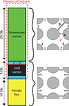 |
Fig. 2. Representation of the system and the boundary conditions. |
The rod diameter is 26.7 mm and the rod pitch is 35.6 mm which gives a pitch to diameter ratio of 1.33. These are the same dimensions as in the CALIFS experimental test section. The hydraulic diameter of the flow in the bundle represented in Figure 2 is equal to 27.8 mm. In order to perform a WRLES of the domain of interest, it is necessary to create a mesh in which the first cell is placed inside the viscous sub layer. Considering the complexity of the original geometry, it is necessary to apply small geometric changes to the grid. The geometry of the grid without mixing vanes and with the simplified springs and dimples visualised from above is given in Figure 3. The geometry of the grid section with mixing vanes is given in Figure 4.
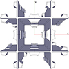 |
Fig. 3. Geometric representation of the grid without mixing vanes, view from above. |
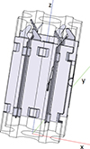 |
Fig. 4. Geometric representation of the grid section with mixing vanes. |
2.2. Boundary conditions
The inlet boundary condition is ensured by the periodic recirculation box illustrated in Figure 2 in which Ubulk = 0.5 m/s is imposed. A constant static pressure is imposed at the outlet of the domain of interest. Two different boundary conditions are imposed at the lateral outlets of the gaps between rods, depending on the part of the domain. In the periodic box as well as in the grid section a symmetry boundary condition is imposed. In the downstream section, a lateral periodic condition is imposed. The presence of such a boundary condition is especially important in the case with mixing vanes in order to reproduce the cross-flow. The lateral periodic boundary condition sets the velocity entering one face equal to the velocity leaving another identical face. Here, the faces linked by the periodic boundary conditions are the faces sharing the same number in Figures 2 and 5.
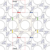 |
Fig. 5. Representation of the periodic mirroring boundary condition of the mixing vanes in CALIFS. |
Figure 5 illustrates the position of the domain within CALIFS 5x5. Such a representation is important to confirm that the use of the mixing vanes does not introduce improper mirroring under this choice of periodic boundary conditions. For example, consider a fluid particle leaving the domain from the lateral outlet numbered 1 towards the subchannel named “top” in Figure 5. The fluid particle then meets the cross-flow created by the mixing vanes in the “top” subchannel. These mixing vanes are in the same configuration as the mixing vanes in the bottom left corner of the computational domain. Therefore, a fluid particle exiting the computational domain through periodic boundary condition number 1 finds itself in a similar cross-flow configuration to the one it would experience if the computational domain also represented the neighboring subchannels of the CALIFS 5x5 test section. However, the periodic boundary condition does not reproduce the flow perfectly as it would if the domain were the full CALIFS 5x5 test section. The unrepresented subchannels of CALIFS in Figure 5 introduce mixing vanes that break the periodicity, as well as the wall of the test section. This can contribute to differences in the cross-flow compared to the periodic boundary conditions that simulate an infinite rod bundle.
2.3. Mesh
The geometries displayed in Figures 3 and 4 allow to build a mesh with y+ between 1 and 5 depending on the geometric complexity. y+ < 1.5 is ensured at the rod walls in the entire “downstream section” represented in green in Figure 2. An estimated Taylor scale λ was calculated with equation (1) in order to choose the edge length for the cells. The calculation is based on the assumption that L = Lint with L the length scale for the large eddies and Lint the integral length scale in the streamwise direction. The value of the spatially averaged integral length scale for Re = 11 200 is Lint = 0.14Dh and for Re = 15 700 is Lint = 0.16Dh. These results come from PIV measurements performed on a 2D plane derived from line (c) of Figure 2 just downstream of the spacer grid with mixing vanes [32]. Hence, a value of Lint = 0.15Dh is chosen here for this estimation.
 (1)
(1)
The Reynolds number based on the length scale ReL is calculated using equation (2) with the estimated turbulent kinetic energy  and the estimated turbulence intensity
  . The Reynolds number Rebulk used to estimate I is the Reynolds number based on the hydraulic diameter and the bulk velocity.
 (2)
(2)
The estimated average Taylor scale is λ = 1.14 mm and the mean edge size for the cells is 0.7 mm, representing 0.6λ. This cell size provide a slightly finer mesh compared to the tetrahedral mesh used for the TrioCFD calculation of the previous benchmark [18], for a calculation with Re = 14 000 instead of Re = 66 000. This estimation of the Taylor scale is only a methodological tool used for mesh construction. The choice of an averaged size of 0.6λ is a compromise between a mesh refinement that ensures the cell size to be of the order of magnitude of λ even in high turbulence intensity zones, and a mesh refinement that limits the computational cost. A verification of the effective Taylor scale based on the results of the calculations is performed in the next section. The meshes are composed of around 40 million cells in the case without mixing vanes and around 50 million in the case with mixing vanes. However, an edge size of 0.6λ is still too high to ensure y + =1. Hence, the use of prism layers at the wall boundary was necessary to enforce this condition. They are composed of 2 sub-layers with a 1.2 stretch factor, for a total thickness of 0.2 mm. This results in a first cell at 0.09 mm from the wall. The meshes are represented in Figure 6.
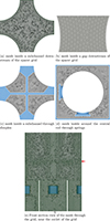 |
Fig. 6. Cross sectional view of the mesh inside a subchannel downstream of the spacer grid (a), inside a gap between two rods (b), inside a subchannel through dimples (c), around the central rod through springs (d). Front section view of the mesh through the grid, near the outlet of the grid (e). The volume cells are represented in grey and the surface cells are represented in blue. |
In Figure 6 the tetrahedrons are represented in grey and appear in 3D whereas the surface cells appearing in Figures 6c and 6d are represented in blue. The red arrow appearing in Figure 6e annotates the conformal passage of the “grid section” to the “downstream section” represented in Figure 2.
Near the wall the distance between two consecutive cells in the x-axis and the z-axis directions is Δx = Δz < 0.7 mm. With the first cell located at 0.09 mm from the wall, yielding y+ = 1, it is possible to estimate that Δx+ = Δz+ < 8 using a simple cross multiplication. Therefore the condition of using a mesh with Δx+ and Δz+ < 100 in order to perform a reliable LES [26] is respected. The prisms in the layer were then divided into 6 tetrahedrons to make the mesh compatible with TrioCFD. The geometry and the mesh were built with the open source software platform SALOME.
2.4. Physical modelling and solver configuration
When performing a LES of an incompressible flow, the velocity U and pressure P fields are decomposed into a filtered part and a residual part. The symbols for the filtered velocity and pressure are  and
and  . The symbol for the residual velocity is
  . The filtered continuity equation (3) and the filtered momentum equation (4) are displayed below, with τij
R
being the residual stress tensor. The residual stress tensor can be decomposed using equation (6) into 2 parts: an isotropic part
. The filtered continuity equation (3) and the filtered momentum equation (4) are displayed below, with τij
R
being the residual stress tensor. The residual stress tensor can be decomposed using equation (6) into 2 parts: an isotropic part  and an anisotropic part τij
r
also called Sub Grid Scale tensor (SGS) [19]. In this decomposition
and an anisotropic part τij
r
also called Sub Grid Scale tensor (SGS) [19]. In this decomposition  is called the residual kinetic energy.
 (3)
(3)
 (4)
(4)
 (5)
(5)
 (6)
(6)
The system of filtered Navier Stokes equations needs to be closed with a model for the SGS. In this study the Wall Adapting Local Eddy Viscosity (WALE) model is chosen for the SGS [27]. With this model the eddy viscosity is modelled with equation (7).
 (7)
(7)
where Sij d defined by equation (8) and calculated using the square of the velocity gradient tensor defined by equations (9) and (10).
 (8)
(8)
 (9)
(9)
 (10)
(10)
The solver configuration is given in Table 1. For both calculations the fluid is liquid water at 20°C and atmospheric pressure.
Chosen configuration with TrioCFD for the solver.
A hybrid Finite Volume Element (FVE) discretisation technique for tetrahedral meshes is employed [33]. This approach produces a discrete finite-element representation of the continuous problem while preserving the flux-balance formulation characteristic of finite-volume methods. In TrioCFD, the velocity is stored at the centres of the tetrahedral faces. Consequently, the number of control volumes used for momentum and scalar transport is roughly twice the number of mesh elements. Pressure is represented using a mixed discretisation, with values defined both at the element centre and at the vertices. This staggered arrangement enhances the coupling between velocity and pressure [34]. To enforce mass conservation, the SOLA projection method introduced by [35] is applied to the velocity field. The robustness and accuracy of this numerical scheme have been demonstrated through benchmark tests for the Navier–Stokes equations [36].
A first calculation is necessary to initialise the periodic box with a duration equal to three times the transit time of a fluid particle through the box. The results are then used to initialise the velocity field inside the box in the actual calculation. In the rest of the domain the calculation is initialised with  m/s. Data acquisition then starts 2 s of simulated physical time after initialisation. This represents approximately 1.3 times the time needed for the passage of a particle of fluid along the domain of interest. The velocity field is then extracted on several planes downstream of the mixing grid every 0.005 s during a physical time long enough to ensure the statistical convergence of first and second order moments. The chosen planes are located at z′=1 Dh, z′=5 Dh, z′=10 Dh and z′=15 Dh.
The calculations were performed with computing HPC and storage resources on the supercomputer Joliot Curie SKL partition using approximately 30 000 cells per processor core. The calculation in the case of the spacer grid without mixing vanes used 1280 cores in parallel and demanded approximately 860 000 CPU hours. The calculation in the case of the spacer grid with mixing vanes used 1664 cores in parallel and demanded approximately 1 120 000 CPU hours.
3. Verification
3.1. Statistical convergence
With the calculation of the Reynolds stress tensor being mandatory to create the colour map, it is necessary to verify the statistical convergence of first- and second-order moments at several locations downstream of the spacer grid. The moments have been verified at several locations: z′=1 Dh, z′=5 Dh, z′=10 Dh and z′=15 Dh and z′=20 Dh. For each location, the averaged velocity field and Reynolds stress tensor are calculated considering the first 1200 time steps, and then the first 1600, 2000, 2400 time steps, plotted over line (a) of Figure 2. Figure 7 shows the results at z′=1 Dh for the Reynolds stress tensor.
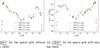 |
Fig. 7. Plot of |

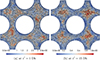 |
Fig. 8.
|


It appears on Figure 7a that the Reynolds stress tensor is sufficiently converged with 2400 time steps in the case of the spacer grid without mixing vanes. The Reynolds stresses are less converged at the transition area between the fine prism layer and the rest of the mesh. This might be due to the rather abrupt transition of cell sizes. Figure 7b shows that after 2400 time steps the 2nd-order moments are perfectly converged. For both cases, the averaged velocity fields are converged. The same conclusion about statistical convergence can be reached at z′=5 Dh, z′=10 Dh and z′=15 Dh and z′=20 Dh.
3.2. Core cell size
It is important to verify that the spatial filter of the LES is in the inertial sub-range of the flow [26]. In order to perform this verification, it is possible to estimate the Taylor microscale for some cells of the mesh and verify that the Taylor microscale in these cells is larger than the maximum edge size of the cell. As mentioned in Section 2, the results are studied mainly over four horizontal planes. With the planes being only one tetrahedron thick along the z-axis, it is not possible to calculate the Taylor scale with a two-point correlation in the streamwise direction. Hence the choice in this study is to estimate the Taylor micro scale using the velocity fluctuations auto-correlation function defined with equation (11). In this equation, u′z represents the velocity fluctuations in the streamwise direction.
 (11)
(11)
To perform the calculation of an autocorrelation function, the data acquisition needs to be sufficiently time-resolved. However, the acquisition of the velocity field over the planes was carried out with a time step of 0.005 s, which can lead to a poor-quality autocorrelation function. Hence, it is important to compare the obtained Taylor microscale between data acquired every 0.005 s and data acquired every 0.0001 s using a segment probe. The segment probes extracted the data at the centre of gravity of the cells intersecting line (a) shown in Figure 2 at several locations: z′=1 Dh, z′=5 Dh, z′=10 Dh and z′=15 Dh. Then, the integration of the autocorrelation function multiplied by the bulk velocity gives an approximate integral lengthscale in the streamwise direction. This integration is presented in equation (12).
 (12)
(12)
The integral length scale Lzz represents the size of the energy containing eddies and is linked to the length scale of the large eddies by equation (13) with Rλ being the Reynolds number based on the Taylor micro scale [19].
 (13)
(13)
The ratio Lzz/L stays between 0.8 and 0.4 and converges towards 0.43 for Rλ above 100 [19]. It is assumed that  for every cell on the planes. The calculation of L allows the determination of ReL, the Reynolds number based on L, following equation (2). The value of ReL then gives the Taylor microscale using equation (1). The ratio max(l)/λ is then calculated for every cell of each plane. The results for the planes at z′=1 Dh and z′=15 Dh are shown in Figure 8 for the case with mixing vanes. The comparison between the Taylor microscale estimated from segment-probe data and that obtained from the plane data extracted along line (a) of Figure 2, at z′=1 Dh for the spacer grid with mixing vanes, is shown in Figure 9. Because the mesh is composed of unstructured tetrahedral cells rather than well-structured and aligned hexahedral cells, it is necessary to define precisely the procedure for selecting the plane cells along line (a). A point is considered to lie on horizontal line (a) if the following conditions are satisfied: |ycell|< 0.3 mm and xcell > 0, with xcell and ycell the coordinates of the gravity center of the cell along the x and y axes.
Figure 8a shows that the maximum edge length lies between 0 and 3.5 times the Taylor scale. Hence, the edge lengths are of the correct order of magnitude for a good LES. However, Figure 8a also shows that a significant proportion of the cells have at least one edge larger than the local Taylor microscale. This issue appears to diminish at z′=15 Dh according to the results in Figure 8b. The analysis of each plane shows that, for the case with mixing vanes, the maxima of max(l)/λ are 3.5, 1.8, 1.3 and 1.0 for z′=1 Dh, z′=5 Dh, z′=10 Dh and z′=15 Dh respectively. The same analysis for the case without mixing vanes gives 2.1, 1.7, 0.98 and 0.81 for z′=1 Dh, z′=5 Dh, z′=10 Dh and z′=15 Dh respectively. With the cell size being equivalent at all distances downstream of the spacer grid, it appears that the estimated Taylor scale increases with the distance from the spacer grid. Figure 9 shows that the Taylor scale calculated from the segment probe data follows the same variations as the Taylor scale calculated from the data extracted on the planes. It also appears from Figure 9 that the differences are of the order of one λ. Therefore, this confirms the conclusions drawn from the results of Figure 8 that the filters used in the calculations are of an appropriate size to perform LES capable of capturing the anisotropy of the flow.

3.3. Viscous boundary layer resolution
It is also important to verify that the simulations are correctly wall-resolved. Figure 10 shows the plot of u+ as a function of y+ at z′=5 Dh, upstream of the grid section, over the line (a) represented in Figure 2. In Figure 10, u+ = < Uz > /uτ with the friction velocity uτ defined by equation (14) and the wall shear stress τw defined by equation (15) [19].
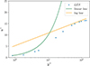 |
Fig. 10. u+ = f(y+) for the fully developed turbulent flow in the gap between rods, z′=5 Dh upstream of the grid section. |
 (14)
(14)
 (15)
(15)
The position z′=5 Dh, upstream of the grid section is chosen for this verification because it represents a fully developed turbulent flow inside a rod bundle. Figure 10 shows that the smallest y+ value is y+ = 0.83, with the second closest being y+ = 1.8. It appears that three of the four points below y+ = 5 do not perfectly fit the theoretical curve u+ = y+. It also appears that the points corresponding to 50 < y+ < 100 are close to the value predicted by the theoretical log law, equation (16) with κ = 0.41 and b = 5.2.
 (16)
(16)
Multiple reasons can explain the discrepancies of the four points inside the viscous sub-layer. At first, the four points might not be perfectly aligned due to the stretched geometry of the near wall cells. The second reason is the gap in size between the cell with y+ = 5 and the next one, having y+ = 17. Indeed, the use of a second order centered scheme for the diffusion, and the use of the Muscl scheme for the convection, imply that the velocity field at y+ = 17 will have a direct impact on the velocity fields calculated on the cells with y+ = 5 and y+ = 4. Despite the differences from the theoretical results, these two calculations show at least six cells before the logarithmic layer. The flow in this region is usually modelled in high-accuracy CFD calculations using this level of geometric fidelity for the spacer-grid design. Hence, the wall resolution of these LES makes it possible to perform new observations on the physical behaviour of the flow downstream of spacer grids.
3.4. Effect of the boundary conditions on the mean flow
It is essential to verify the physical consistency of the results. In this case, the use of a reduced model, with the periodic boundary conditions could have a negative impact on the mean flow velocity. In the case of the flow with mixing vanes, the secondary flow has a specific shape, induced by the presence of the mixing vanes. That shape was often verified and illustrated in the literature [12, 28, 29]. Therefore, it is important to verify that the shape of the secondary flow is the same as the shape observed inside the entire rod bundles. Figure 11 shows the vector representation of the non-streamwise components of the averaged velocity field at z′=5 Dh, with mixing vanes.
Figure 11 illustrates that the flow shows the diagonal cross flow pattern, observed often in the literature on non-reduced models. Therefore, the combination of the reduced geometry and the chosen boundary conditions seems to reproduce the physical behaviour of the averaged velocity field inside a fuel assembly.
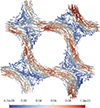 |
Fig. 11. Vector representation of the non streamwise components of the averaged velocity field, at z′=5 Dh with mixing vanes. In the figure, the colour-map represents the scale of secondary flow velocity magnitude normalised by the bulk velocity. |
4. Comparison with experimental results
The last element that can confirm the reliability of the numerical results is the comparison with available experimental results from the CALIFS 5x5 test section [32]. The comparison is made with PIV results at a Reynolds number of 14 000, over the line (c) represented in Figure 2, at z′=1 Dh, for both cases. The averaged velocity fields are plotted in Figure 12 for the case without mixing vanes, and Figure 13 for the case with mixing vanes. The Root Mean Square (RMS) of the velocity fluctuations is plotted in Figure 14 for the case without mixing vanes and Figure 15 for the case with mixing vanes. Line (c) is located at a distance of 2 mm from the wall of the central rod. A 1 mm-thick laser sheet was used during the CALIFS 5x5 PIV measurements, with an estimation of 3% for the uncertainty on the particles displacements [32].
Figure 12a shows a good agreement of the streamwise velocity field between the experimental and the numerical results in the case without mixing vanes. The maximum of the relative error to the experiment is 12%, and the averaged discrepancy is 6%. Figure 12b also shows that the numerical and experimental results for the averaged lateral velocity field follow the same variations. Figure 12b also shows that the lateral velocity profiles are neither symmetrical in the experiment nor in the calculation. Indeed, the position of the line (c) is close to the rod and not in the middle of the gap. Hence, the spring and the dimple influencing the flow in the top and bottom gaps might influence the lateral velocity field calculated over line (c), just downstream of the spacer grid. At last, it appears from Figures 14a and 14b that the numerical values of the RMS of the velocity fluctuations are in really good agreement with the experimental data.
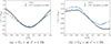 |
Fig. 12. Plot of |


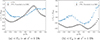 |
Fig. 13. Plot of |


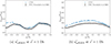 |
Fig. 14. Plot of |


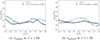 |
Fig. 15. Plot of |


The proximity between experimental and numerical results is lower in the case with mixing vanes. Figure 13a shows that the calculated averaged velocity fields along the streamwise direction are the same order of magnitude as the measured ones. The same observation can be made for the averaged velocity fields in the spanwise direction, as shown in Figure 13b. The plots of Figure 13 seem to show that the numerical results and the experimental results follow the same variations, with a positional offset of the maxima and minima along the Oy axis. The same observations are made with the plots in Figure 15. Figures 15a and 15b show that the calculated RMS of the velocity fluctuations along the streamwise and spanwise directions are in correct agreement with the results from the CALIFS experiments, but also show an offset in the positions of the variations. The possible sources of error are the use of a reduced geometry in the simulations, with periodic boundary conditions, and the differences in spatial resolutions between the LES and PIV.
The comparisons with the CALIFS experimental results show that both simulations give physically consistent results and are accurate enough to ensure the reliability of the following analysis, concerning the turbulence anisotropy of the flow.
5. Comparison of flow metrics
Some flow metrics of both cases are compared in this section. The different physical quantities are plotted over the line (b) of Figure 2. A point is considered to belong to line (b) if |y − ax|< ϵ, with |y = ax| being the equation of the line in the (0, x, y, z) set of coordinates, and ϵ = 0.5 mm being the line thickness. The line thickness can lead to points with the same x-axis value R/Dh, on the graph but different values along the y-axis. The cross-flows are compared in Figure 16, and the turbulence intensities are compared in Figure 17.
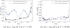 |
Fig. 16. Plot of |Ux + Uy|/∥U∥, over the line (b) at z′=1 Dh (a), z′=10 Dh (b). |
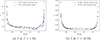 |
Fig. 17. Plot of I, over the line (b) at z′=1 Dh (a), z′=10 Dh (b). |
Figure 16a shows that, at z′=1 Dh, the cross-flow is more significant in the presence of mixing vanes than in their absence. At z′=1 Dh, the cross-flows of both cases are equivalent in the vicinity of the rods. Away from the rod vicinity, the variations in cross-flows, and the values taken, are different between the two cases. In the case with mixing vanes, the cross-flow rises to attain a local maximum around R/Dh = 0.7, then diminishes to reach a minimum at R/Dh = 0.9, and then rises again to attain another local maximum at R/Dh = 1.1. These variations are in agreement with the expected form of the cross-flow just downstream of a grid with mixing vanes, as observed in Figure 11. The two local maxima correspond to the two strong streams going in opposite directions, shown in red in the right corner of Figure 11. The local minimum corresponds to the area trapped between the two opposite streams. At z′=1 Dh, the cross-flow in the case without mixing vanes rises slowly in the subchannel with increasing distance from the central rod. At z′=1 Dh, the cross-flow is between 4 and 8 times greater in the subchannel in the case with mixing vanes, except at the local minimum, where the two cross-flows are equivalent. At z′=10 Dh, Figure 16b shows that, in both cases, the cross-flows are of the same order of magnitude. A local minimum is reached at the limit of the rod vicinity, at R/Dh = 0.6, then it rises to a local maximum at approximately R/Dh = 0.7, and then slowly decreases until R/Dh = 1.2 at z′=10 Dh.
According to Figure 17, the variations, and magnitude, of turbulence intensity show fewer differences between the cases than the cross-flows. At z′=10 Dh, Figure 17b shows nearly identical values and variations of turbulence intensity between the two cases. At z′=1 Dh, the turbulence intensity in the case without mixing vanes passes through a local maximum at R/Dh = 0.9 and a local minimum at R/Dh = 1.1. As for the case with mixing vanes, it follows the same variations of turbulence intensity as at z′=10 Dh. For both cases, the value of the turbulence intensity is around 0.8 at the rod walls and 0.2 in the subchannel at z′=1 Dh. The turbulence intensity then decreases to 0.4 at the rod walls, and progressively to 0.05 in the subchannel at z′=10 Dh.
It is also interesting to compare other turbulence quantities, like the integral length scale in the streamwise direction, Lzz, as well as the decay rate, τ. τ is defined by equation (17) [19]. However, the turbulent dissipation rate, ϵ, cannot be directly calculated from the results of LES. Therefore, τ is estimated using equation (18), derived from equation (19) [19], with L estimated using equation (13). As for Lzz, it is calculated with equation (12). The data for the integral length scale and the decay rate are presented in Figures 18 and 19.
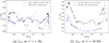 |
Fig. 18. Plot of Lzz, over the line (b) at z′=1 Dh (a), z′=10 Dh (b). |
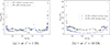 |
Fig. 19. Plot of τ, over the line (b) at z′=1 Dh (a) z′=10 Dh (b). |
 (17)
(17)
 (18)
(18)
 (19)
(19)
Figure 18 shows strong differences between the two cases in the variations of the estimated values of Lzz at each position downstream of the spacer grid. Figure 18a shows that, at z′=1 Dh, Lzz evolves between 0.05 Dh and 0.20 Dh and takes equivalent values in the subchannel, and in the rod vicinity. Figure 18b shows a different behaviour with values of Lzz higher in the rod vicinity than in the subchannel and taking higher values up to Lzz = 0.75 Dh in the case with mixing vanes. The differences between both cases highlight the creation of variations in size and shape for the vortex structures, depending on the presence of the mixing vanes. However, the analysis of the turbulence intensity seems to indicate that these different vortex structures are responsible for the same level of turbulence intensity.
Figure 19a shows that τ evolves between  and
and  for both cases, at z′=1 Dh. For both cases, the values above
  are reached in the immediate vicinity of the rods. In the subchannel, the variations are stronger in the case with mixing vanes, with local minima and maxima more pronounced than in the case without mixing vanes. At z′=10 Dh, Figure 19b shows that the variations of τ strongly diminish in the subchannel in the case with mixing vanes. The observations made for the case without mixing vanes are different, with a local maximum appearing at R/Dh = 0.7, reaching higher values than in the case with mixing vanes. As for the overall values of τ it appears from Figure 19b that they are higher than the values reached at z′=1 Dh. The higher values for τ in the case without mixing vanes seem to indicate that, at z′=10 Dh, the vortex structures decay more slowly than in the case with mixing vanes.
6. Post-processing method for the analysis of turbulence anisotropy
This section briefly explains the method used previously in the literature in order to visualise anisotropy using the calculation of eigenvalues [22]. The method is more thoroughly explained in the literature [23]. The application of the post-processing to the results of a LES, starts with the hypothesis that the filtered velocity from the simulation is equal to the actual velocity field:  . A RANS post-processing of this velocity field is then performed. Since the data acquisition period is sufficiently long to ensure the convergence of both the averaged velocity field and the Reynolds stress tensor, it is assumed that time-averaging the data across all time steps is equivalent to statistical averaging. The Reynolds stress tensor is then separated into an isotropic part
  , and an anisotropic part aij, following equation (20), with δij being the Kronecker symbol. It is then possible to normalise aij and obtain
  . Therefore, bij is obtained from the Reynolds stress tensor using equation (21).
 (20)
(20)
 (21)
(21)
The eigenvalues, λ1, λ2, λ3, of bij are then calculated, considering that λ1 > λ2 > λ3. By definition of bij, the sum of its eigenvalues is null equation (22). From these eigenvalues, is it possible to introduce three weights, which characterise the anisotropy of the flow. The three weights C1c, C2c and C3c are defined by equations (23)–(25).
 (22)
(22)
 (23)
(23)
 (24)
(24)
 (25)
(25)
By definition of the weights, and using equation (22), it is possible to write equation (26). The weights are then used as a Red-Green-Blue triplet, which allows the visualisation of the turbulent anisotropic behaviour of the flow on a colour map.
 (26)
(26)
Depending on the values of C1c, C2c and C3c, three limit states can be defined:
-
State 1: C1c = 1, C2c = 0 and C3c = 0.
Equations (22)–(25) then give
 ,
,  and
and  . Therefore equation (21) gives < u′1u′1 > = 2k and < u′2u′2 > = < u′3u′3 > = 0 in the coordinate system associated to the eigenvalues. Hence, the flow is anisotropic with the velocity fluctuations strong in one direction and null in the two others. This limit state appears in red, and is represented as x1C in the colour maps.
 -
State 2: C2c = 1, C1c = 0 and C3c = 0.
Equations (22)–(25) then give
 ,
,  and
and  . Therefore equation (21) gives < u′1u′1 > = < u′2u′2 > = k and < u′3u′3 > = 0 in the coordinate system associated to the eigenvalues. Hence, the flow is anisotropic with the velocity fluctuations strong in two directions and null in the last one. This limit state appears in green, and is represented as x2C in the colour maps.
 -
State 3: C3c = 1, C1c = 0 and C2c = 0.
Equations (22)–(25) give λ1 = λ2 = λ3 = 0. Therefore bij is null and the flow is isotropic. This limit state appears in blue, and is represented as x3C in colour the maps.
This method was used on the DNS results of a the flow inside a 5x5 bare rod bundle and Figure 20 (Fig. 13 in the original article) was obtained [22].
 |
Fig. 20. Barycentric map of componentality contours for a 5x5 bare rod bundle, DNS results from [22]. |
In Figure 20, the authors added an exponent, and an offset, to each of the weights to modify the colour-mapping in order to be able to better distinguish the transitions between the three limiting states mentioned before [22]. However this does not change the reading method of Figure 20. The red colour appearing in the walls vicinity in Figure 20 indicates that the flow in these areas is anisotropic, with one-component velocity fluctuations. The blue colour present in the gaps and the subchannel indicates an isotropic flow, in these areas. The green colour appearing in the gaps between the rod and the bundle walls indicates an anisotropic flow, with velocity fluctuations along two components. In the following sections the colour maps presented do not have the offset or the exponent used in Figure 20.
7. Anisotropy analysis without mixing vanes
In this part, the results obtained using the post-processing method of Section 6 in the case without mixing vanes, are presented. The colour maps are first analysed and then the focus is put on the plots over the line (b), introduced in Figure 2.
7.1. Physical analysis over the planes
The colour maps, obtained from the calculation of eigenvalues of the anisotropic part of the Reynolds stress tensor, are plotted in Figure 21. The results of the calculation without mixing vanes, on planes z′=1 Dh, z′=5 Dh, z′=10 Dh and z′=15 Dh are shown respectively in Figures 21a–21d. Figure 21a shows an overall strongly anisotropic flow on the plane at z′=1 Dh. It appears from the green colour surrounding the rods that the velocity fluctuations near the rod wall are strong in two different directions. The blue colour forming a grid-like form indicates that the flow is close to an isotropic state in the middle of the gaps and the subchannels. The flow is also strongly anisotropic in the regions appearing in magenta on the map. In these regions the flow is not in one of the three limit states but it is between isotropy and anisotropy with velocity fluctuations stronger in one direction.
Figure 21c shows with the red colour a strong anisotropy with velocity fluctuations along one component at the rod wall, at z′=10 Dh. The blue colour present in a large area is indicates a nearly isotropic flow in the majority of the subchannel and the gaps between rods. At last, the cyan colour surrounding the red colour on the map indicates an in-between state, with the velocity fluctuations being non zero but lower in one direction than the two others.
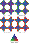 |
Fig. 21. Anisotropy componentality contours at, z′=1 Dh (a), z′=5 Dh (b), z′=10 Dh (c), z′=15 Dh (d), in the case of the grid without mixing vanes and the chosen colour mapping (e). |
The results at z′=5 Dh are presented in Figure 21b. The colour map shows the green colour turning to red for some cells in the logarithmic sub-layer. This indicates that the flow is also anisotropic in the rod vicinity but the velocity fluctuations appear to evolve between one and two components. The magenta colour present in Figure 21a has been replaced by the blue colour indicating a large area of nearly isotropic flow. Hence, the flow is nearly isotropic in the subchannels and in the gaps between rods at z′=5 Dh. Therefore, Figure 21b appears to be a transitional state between the results of Figures 21a and 21c.
At last, Figure 21d shows the results at z′=15 Dh. The results at z′=15 Dh are similar to the results at z′=10 Dh. However, on this map, the red portions in the rod vicinity have become larger. Therefore, the proportion of the domain in which the flow is isotropic decreases, and the proportion in which the flow is anisotropic, with velocity fluctuations along one component, increases.
7.2. One-dimensional profiles
In this sub-section the Reynolds stress tensor and the weights C1c, C2c and C3c are plotted over the line (b) from Figure 2. The considered terms of the Reynolds stress tensor are: < u′ru′r> , < u′θu′θ> and < u′zu′z> with (O, r, θ, z) the polar set of coordinates associated to line (b), where O is the centre of the central rod. Hence < u′ru′r> represents the Reynolds stress tensor in the rod normal direction, and < u′θu′θ> represents the Reynolds stress tensor in the direction orthogonal to the rod normal direction. This last direction will be mentioned later in the text as being the “span-wise” direction. All the terms of the Reynolds stress tensor will be normalised by  . A point is considered as belonging to line (b) if |y − ax|< ϵ with |y = ax| being the equation of the line in the (0, x, y, z) set of coordinates and, ϵ = 0.5 mm being the line thickness. The line thickness can lead to points with the same x-axis value R/Dh on the graph but different values along the y-axis. The results are presented in Figure 22.
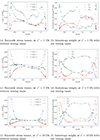 |
Fig. 22. Reynolds stress tensor (a) and Anisotropy weight (b) plot over the subchannel line b from Figure 1 at z′=1 Dh. Reynolds stress tensor (c) and Anisotropy weight (d) plot over the subchannel line b from Figure 1 at z′=5 Dh. Reynolds stress tensor (e) and Anisotropy weight (f) plot over the subchannel line b from Figure 1 at z′=10 Dh. |
It appears in Figure 22a that the maximum of the normalised Reynolds stress in one component reaches 0.21. The sum of the normalised Reynolds stresses remains greater than or equal to 0.15 everywhere for 0.5 < R/Dh < 1.3. Hence it appears on Figure 22 that the mixing grid highly enhances the velocity fluctuations and the turbulence kinetic energy close to the grid. A closer look at Figure 22a shows that the span-wise and the streamwise velocity fluctuations are strong at the walls and decrease in the subchannel. The rod-normal velocity fluctuation is null at the rod wall and increases slowly in the subchannel. Despite this increase the normal component of the velocity fluctuations remains lower than the streamwise velocity fluctuations for 0.6 < R/Dh < 1.2. It appears that the span-wise velocity fluctuations are as strong as the streamwise velocity fluctuations near the rod boundary at z′=1 Dh. The close values between the streamwise and the span-wise velocity fluctuations explain the observations in the rod vicinity made from Figure 21a. The in between state represented in magenta in Figure 21a can be better understood by analysing Figure 22b at 0.6 < R/Dh < 0.8 and 1.0 < R/Dh < 1.2. It appears in these areas of the plot that C1c and C3c are both stronger than C2c which is nearly zero. Figure 22a shows that the span-wise and rod-normal Reynolds stresses are nearly equal, with a value that is approximately half the value of the Reynolds stress in the streamwise direction for 0.6 < R/Dh < 0.8 and 1.0 < R/Dh < 1.2. Figure 22b also shows a maximum value for C3c of 0.8. This value is characteristic of a flow close to an isotropic state.
It appears from Figures 22a and 22c that the sum of the normalised Reynolds stresses goes from a maximum of 0.40 at z′=1 Dh to 0.06, at z′=5 Dh. Hence there is a strong loss of turbulent kinetic energy compared to the results at z′=1 Dh. The variations of Reynolds stresses from Figure 22c are also different in comparison with the results from Figure 22a. The streamwise component increases sharply in the rod vicinity then decreases with the distance from the rods. The span-wise component increases more slowly than the streamwise component and decreases far away from the rods. The normal component starts with a null value at the walls and increases in the subchannel. In the case of Figure 22c the span-wise velocity fluctuations remain lower than the streamwise velocity fluctuations for R/Dh < 0.5. Figure 22d has a maximum value for C3c of 0.7. This is characteristic of a nearly isotropic flow. The portion of Figure 22d with C3c being above 0.6 is larger than in Figure 22b, confirming that a larger area of the flow is in a nearly isotropic state. A more thorough analysis of Figure 22d shows that C2c is greater than C1c for the three cells that are the closest to the central rod. Once these three cells are past, C1c becomes greater than C2c for the next 4 cells due to the two large extreme values of < u′zu′z> visible in Figure 22c. Finally, the cyan colour appearing in Figure 21b corresponds to a transitional state with C2c larger than C1c between the rod vicinity and the large nearly isotropic area. In this transitional state C2c = 0.6 on Figure 22d. This corresponds to < u′θu′θ> = < u′zu′z> being greater than a non-zero < u′ru′r> in Figure 22c.
Figure 22e shows results similar to Figure 22c. The sum of the normalised Reynolds stresses represents approximately 0.06 close to the rod and approximately 0.03 in the middle of the subchannel. Hence turbulence decay between z′=5 Dh and z′=10 Dh is less important than the decay between z′=1 Dh and at z′=5 Dh. Figure 22e shows that the Reynolds stresses follow the same variations as at z′=5 Dh and at z′=10 Dh. The streamwise Reynolds stress is 5 times larger than the span-wise Reynolds stress in the rod vicinity at z′=10 Dh. For 0.7 < R/Dh < 1.1 the Reynolds stresses are of the same order of magnitude and Figure 22f confirms that the flow is nearly isotropic in this portion of the subchannel. According to Figure 22e the span-wise Reynolds stress never exceeds the streamwise Reynolds stress unlike in the cases z′=1 Dh and at z′=5 Dh. Figure 22f shows that the closest point to the central rod shows C2C greater than C1C. The rest of the points in the vicinity of the central rod have C1C greater than C2C. Figure 22f confirms the presence of a transitional area similar to the one found in Figure 22d, allowing the transition between the anisotropy in the rod vicinity and the isotropic part of the flow.
8. Anisotropy analysis with mixing vanes
The post-processing method of Section 6 is now applied to the results from the cases with mixing vanes. As in Section 7, the analysis starts on the colour maps and then moves on to the plots over the line (b) from Figure 2.
8.1. Physical analysis over the planes
The colour maps obtained from the results of the calculation with mixing vanes on planes at z′=1 Dh, z′=5 Dh, z′=10 Dh, and z′=15 Dh are given respectively in Figures 23a–23d.
Figure 23a shows the anisotropy of the flow at z′=1 Dh. The flow appears to be mainly anisotropic with some scattered isotropic areas appearing in blue on the map. The green colour around the rods indicates that the velocity fluctuations evolve along two components in the rod vicinity, as was the case for Figure 21a. It is possible to distinguish cyan eddy-shaped patterns in the subchannels of Figure 23a. These patterns have an ellipsoid shape and follow the inclinations of the mixing vanes.
Figures 23b and 21b are much more alike than Figures 23a and 21a. Figure 23b shows the same mix of green and red in the rod vicinity; indicating a transition occurring at z′=5, with the flow passing from velocity fluctuations along two components to velocity fluctuations along one component. The large areas of blue colour in Figure 23b also indicate that a large part of the section showcases a nearly isotropic turbulent flow. However, unlike in Figure 21b some anisotropic areas appear in each of the subchannels.
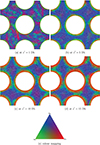 |
Fig. 23. Anisotropy componentality contours at, z′=1 Dh (a), z′=5 Dh (b), z′=10 Dh (c), z′=15 Dh (d) and the chosen colour mapping (e). |
Figure 23c shows the flow anisotropy at z′=10 Dh. There are again great similarities between the results with mixing vanes from Figure 23c and its no mixing vanes counterpart from Figure 21c. At z′=10 Dh, a strong red colour appears in the vicinity of the rod, indicating a strongly anisotropic flow with velocity fluctuations along a single component. There are also large blue areas indicating a nearly isotropic flow. However, the presence of the magenta areas indicates that the flow remains anisotropic in the subchannels, as in Figure 23b.
Figure 23d shows the flow anisotropy at z′=15 Dh. The analysis is the same as that for Figure 23c. The red areas in the rod vicinity are larger at z′=15 Dh than at z′=10 Dh. However the magenta anisotropic areas in the subchannels are diminished compared to Figure 23c. The analysis of the 4 maps seems to indicate that the patterns observed in the subchannel at z′=1 Dh propagate further downstream and are responsible for the flow anisotropy in the subchannel up to at least 15 Dh.
8.2. One-dimensional profiles
In this subsection the Reynolds stress tensor and the anisotropy weights are plotted over the line (b) of Figure 2. The plotted components of the Reynolds stress tensor are the same as in Section 7.2, using same cylindrical coordinates system. The results are given in Figure 24.
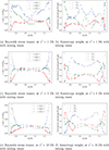 |
Fig. 24. Reynolds stress tensor (a) and Anisotropy weight (b) plot over the subchannel line, z′=1 Dh in the case of the grid with mixing vanes. Reynolds stress tensor (c) and Anisotropy weight (d) plot over the subchannel line, z′=5 Dh in the case of the grid with mixing vanes. Reynolds stress tensor (e) and Anisotropy weight (f) plot over the subchannel line, z′=10 Dh in the case of the grid with mixing vanes. |
Figure 24a indicates that the maximum of the normalised Reynolds stress in one component reaches 0.23. The sum of the normalised Reynolds stresses remains greater than or equal to 0.15 everywhere for 0.5 < R/Dh < 1.3. The Reynolds stress in the streamwise direction increases in the vicinity of the rods, then remains nearly constant around R/Dh = 0.6 and then strongly decreases around R/Dh = 0.7 to reach its minimum in the middle of the subchannel. For values of R/Dh > 0.8, the Reynolds stress in the streamwise direction steadily increases to reach its maximum in the rod vicinity and then plummets, getting closer to the rod wall. The Reynolds stress in the span-wise direction is nearly equal to the Reynolds stress in the streamwise direction near the central rod wall but small near the other rod wall. However, it drops faster in both cases than the Reynolds stress in the streamwise direction in order to reach its minimum in the middle of the subchannel. The normal component of the Reynolds stress is null in the rod vicinity and increases slowly up until R/Dh = 0.6. It then remains nearly constant for 0.6 < R/Dh < 0.8 and increases its maximum in the subchannel. The profile of the Reynolds stress in the rod normal direction then follows a symmetrical pattern for R/Dh > 0.9. The three Reynolds stresses are never equivalent in the subchannel. The maximum value reached by C3c is around 0.7 in Figure 24b.
Figure 24c shows a maximum of normalised Reynolds stress at less than 0.05. Hence, the turbulent kinetic energy of the flow has decreased significantly when passing from 1 Dh to at z′=5 Dh. Figure 24c shows a high streamwise component of the Reynolds stress tensor at the walls that diminishes in the subchannel. The span-wise component remains greater than the normal component at the rod wall but is significantly lower than the streamwise component. In the subchannel, the three components are close. Figure 24d has a maximum value for C3C around 0.8 which is close to isotropy. However C3C is below 0.6 for  . Hence, the flow is not isotropic in the central part of the subchannel. Figure 24d also shows similar results to Figure 22d regarding the behaviours of C1c and C2c in the rod vicinity for
  and
and  . In these zones the first one or two cells have a high value of C2c, which then plummets to a value lower than C1c. Then C2c increases to 0.5 again in the transition between the rod vicinity and the isotropic part of the flow.
The nature of the variations of the Reynolds stress tensor in Figure 24e is nearly identical to the variations in Figure 24c. However, the numerical values are different. Figure 24e shows a single point with C2C greater than C1C close to the rods. After this first point C1C is the strongest of the three weights until the transition zone. After this transition zone C3C becomes the strongest in the range  . The maximum value reached for C3C is 0.7. C3C lies between 0.4 and 0.5 for 0.8 < R/Dh < 1.0 indicating that the flow is far from isotropy in the middle of the subchannel at z′=10 Dh.
9. Discussion
The results of the calculations highlighted a lot of differences between the flows downstream of the two configurations of spacer grids. At first it appeared that the cross-flow close to the grid is far more important in the case with mixing vanes, especially in the subchannel. The differences in the behaviour of the cross-flow remain with the distance away from the grid, however, the magnitude of the cross-flow compared to the norm of the velocity field are equivalent between the cases at z′=10 Dh. Although the cross-flows are different, very few differences appear between the cases when analysing the turbulence intensity of the flow. This seems to confirm the equivalent orders of magnitude observed for the turbulent kinetic energy and Reynolds stress tensor of the flow analysed in the last two sections. Important differences appear in the analysis of the integral length scale of the flow at every location downstream of the spacer grid. These differences, coupled with the analysis of turbulence intensity, seem to indicate that the vortex structures created in both cases are different and propagate differently but generate an equivalent level of turbulence intensity within the flow. At last the analysis of the decay rate tends to show that the vortex structures generated downstream of a spacer grid decay faster with the distance away from the grid in the case without mixing vanes.
The results analysed in this study confirm that the flow inside a rod bundle downstream of a spacer grid is highly anisotropic. The flow anisotropy differs with numerous parameters such as the type of grid (without or with mixing vanes) as well as the distance from the grid. The anisotropic behaviour of the flow is also different depending on the region of interest, whether it is inside the subchannel, the gaps between rods or the rod vicinity.
The anisotropic behaviour of the flow close to the grid is very different from the case without a grid. The results at z′=1 Dh show that, in the case without mixing vanes, the flow remains nearly isotropic only in a short area located in the middle of the subchannels and in the middle of the gaps. In the presence of the mixing vanes, the grid creates anisotropic patterns linked to the mixing vanes’ orientations in the subchannels. These patterns are delimited by zones with strong streamwise velocity fluctuations, weaker span-wise velocity fluctuations, and even weaker rod-normal velocity fluctuations. Hence, the flow is anisotropic in the entire subchannels at z′=1 Dh in the case of a spacer grid with mixing vanes. The results also show that in this case the flow is also anisotropic in the gaps between rods. Whether the grid has mixing vanes or not, the flow in the vicinity of the rods is anisotropic with velocity fluctuations equivalent in the streamwise and the span-wise directions at z′=1 Dh. The observation of strong velocity fluctuations in two components in the rod vicinity might be important for local estimations of heat transfer at the rod walls or rod excitation forces. All of these observations constitute yet another argument for the use of a non-linear eddy viscosity model when performing unsteady RANS CFD calculations of the flow inside a rod bundle downstream of a spacer grid.
The differences with the case without a grid only diminish with the distance from the grid. Whether the grid has mixing vanes or not, the flow is isotropic in the entire gaps by z′=5 Dh. This is similar to the case without a grid. In the case without mixing vanes, the flow becomes isotropic in the entire subchannel, as it does in the case without a grid. In the case with mixing vanes, the anisotropic patterns observed at z′=1 Dh propagate downstream, leaving the flow in an anisotropic state at z′=5 Dh. These anisotropic patterns then propagate further downstream of the grid. Although these anisotropic patterns seem to decay with the distance from the grid, the anisotropy remains in the middle of the subchannels up to z′=15 Dh. The flow in the rod vicinity tends to shift from velocity fluctuations strong along two components to velocity fluctuations strong along one component at z′=5 Dh, with or without mixing vanes. By z′=10 Dh, the velocity fluctuations in the rod vicinity are stronger in the streamwise direction than in the other two, as they are in the case without a spacer grid.
The analysis of flow metrics and turbulence anisotropy together seems to show that the mixing vanes are responsible for the creation of different turbulent structures compared with those observed without mixing vanes, as well as a stronger cross-flow. These turbulence structures are not responsible for an increase in turbulence intensity or turbulent kinetic energy. However, these turbulence structures decay less rapidly than in the case without mixing vanes. This slower decay might lead to slower breakdown of the large anisotropic eddies into smaller isotropic eddies. This could be linked to the observation of turbulence anisotropy in the subchannels, which is only observed in the case with mixing vanes.
10. Conclusion
The WRLES of a reduced model of the CALIFS 5x5 test section has been performed at Re = 14 000 with and without mixing vanes on the grid. For each simulation the velocity field was extracted on several planes at different distances downstream of the spacer grid. Several checks were then performed to ensure the reliability of the results. After this, the turbulent anisotropy of the flow was characterised for both cases using the calculation of the Reynolds stress tensor eigenvalues.
The results show a strong influence of the grid on the turbulence anisotropy at z′=1 Dh. This impact is the same with or without mixing vanes in the rod vicinity. Close to the rods, the velocity fluctuations are equivalent along the streamwise and span-wise components but remain null on the rod-normal component. The influence of the grid on the turbulence anisotropy becomes negligible by z′=10 Dh after the passage of the grid without mixing vanes. In the case with mixing vanes, the grid continues to have an impact on the turbulence anisotropy in the subchannels at least for the first at z′=15 Dh.
Some possible perspectives on this work would be to assess the impact of the choices made on the geometry used to perform the calculation. In the future, the same numerical methodology could be applied to simulate the entire CALIFS 5x5 domain in order to assess the impact of using a shorter domain on the accuracy of the results presented. Another possibility would be to extend the rod-bundle length downstream of the spacer grid and apply a periodic boundary condition that returns the outflow to the inlet of the computational domain. The results of such calculations could make it possible to assess the influence of the upstream spacer grid on the flow within the domain of interest in the CALIFS 5×5 test section.
At last, numerous ways could be explored to complete this work in the process of explaining the discrepancies observed between LES results and experimental results in the previous benchmarks. For example, the size of the filter and the use of a wall model could affect the calculation of pressure fluctuations at the rods walls. Another study assessing the impact of mesh refinements and coarsening will be conducted in order to confirm of refute these hypotheses. The results of this study also raises several interrogations on the impact of the flow anisotropy in the rod vicinity for the numerical simulations of heat transfer and excitation forces downstream of spacer grids.
Funding
This research did not receive any specific funding.
Conflicts of interest
The authors declare that they have no competing interests to report.
Data availability statement
Data associated with this article cannot be disclosed due to legal reason.
Author contribution statement
Hugues Charton: Conceptualisation, Methodology, Formal analysis, Investigation, Data Curation, Writing – Original Draft, Writing – Review and Editing. Emmanuel Lo Pinto: Conceptualisation, Resources, Methodology, Supervision, Writing – Review and Editing, Project administration, Funding acquisition. Guillaume Ricciardi: Conceptualisation, Methodology, Supervision, Writing – Review and Editing.
Acknowledgments
This work is supported by project ASSEMBLAGE within the Energy Division of CEA (DES). The authors are grateful for the financial support of Electricité de France (EDF) and Framatome. This project was provided with computing HPC and storage resources by GENCI at TGCC thanks to the grant 2024-A0172A15660 on the supercomputer Joliot Curie SKL partition.
References
- Ricciardi, G., Faucher, V., Rossi, L., François, F., Collard, B., Bardet, P., Review of spacer grid to rod fretting in pressurized water reactor, Nucl. Eng. Des. 418, 112901 (2024), https://doi.org/10.1016/j.nucengdes.2024.112901 [Google Scholar]
- Chang, S.-K., Kim, S., Song, C.-H., Turbulent mixing in a rod bundle with vaned spacer grids: OECD/NEA–KAERI CFD benchmark exercise test, Nucl. Eng. Des. 279, 19 (2014), https://doi.org/10.1016/j.nucengdes.2014.05.013 [Google Scholar]
- Lee, J.R., Kim, J., Song, C.-H., Synthesis of the turbulent mixing in a rod bundle with vaned spacer grids based on the OECD-KAERI CFD benchmark exercise, Nucl. Eng. Des. 279, 3 (2014), https://doi.org/10.1016/j.nucengdes.2014.03.008 [Google Scholar]
- Rashkovan, A., McClure, D., Novog, D.R., Examination of separate-effect and integral phenomena within a grid spacer with mixing vanes: Results for the MATiS-H OECD/NEA benchmark exercise, Nucl. Sci. Eng. 177, 141 (2014), https://doi.org/10.13182/NSE13-4 [Google Scholar]
- Cinosi, N., Walker, S.P., Bluck, M.J., Issa, R., CFD simulation of turbulent flow in a rod bundle with spacer grids (MATIS-H) using STAR-CCM+, Nucl. Eng. Des. 279, 37 (2014), https://doi.org/10.1016/j.nucengdes.2014.06.019 [Google Scholar]
- Podila, K., Rao, Y., CFD modelling of turbulent flows through 5 × 5 fuel rod bundles with spacer-grids, Ann. Nucl. Energy 97, 86 (2016), https://doi.org/10.1016/j.anucene.2016.07.003 [Google Scholar]
- Batta, A., Class, A.G., CFD study of isothermal water flow in rod bundle with split-type spacer grid, in SNA + MC 2013 – Joint International Conference on Supercomputing in Nuclear Applications + Monte Carlo (EDP Sciences, Paris (France), 2014), p. 01201, https://doi.org/10.1051/snamc/201401201 [Google Scholar]
- Huang, Y., Cai, J., Research on prediction of turbulence intensities of 5-by-5 rod bundle with a split-vane spacer grid, Prog. Nucl. Energy 152, 104354 (2022), https://doi.org/10.1016/j.pnucene.2022.104354 [Google Scholar]
- Wang, Y., Wang, M., Ju, H., Zhao, M., Zhang, D., Tian, W., Liu, T., Squire, S., Su, G.H., CFD simulation of flow and heat transfer characteristics in a 5×5 fuel rod bundles with spacer grids of advanced PWR, Nucl. Eng. Technol. 52, 1386 (2020), https://doi.org/10.1016/j.net.2019.12.012 [Google Scholar]
- Mistry, H., Numerical investigations of flow in nuclear fuel assembly with spacer grid and OpenFOAM validation, Kerntechnik 88, 141 (2023), https://doi.org/10.1515/kern-2022-0109 [Google Scholar]
- Peña-Monferrer, C., Muñoz-Cobo, J.L., Chiva, S., CFD turbulence study of PWR spacer-grids in a rod bundle, Sci. Technol. Nucl. Install. 2014, 1 (2014), https://doi.org/10.1155/2014/635651 [Google Scholar]
- Chang, D., Tavoularis, S., Hybrid simulations of the near field of a split-vane spacer grid in a rod bundle, Int. J. Heat Fluid Flow 51, 151 (2015), https://doi.org/10.1016/j.ijheatfluidflow.2014.07.005 [Google Scholar]
- Končar, B., Košmrlj, S., Simulation of turbulent flow in MATIS-H rod bundle with split-type mixing vanes, Nucl. Eng. Des. 327, 112 (2018), https://doi.org/10.1016/j.nucengdes.2017.12.017 [Google Scholar]
- Faucher, H., Palancher, H., Ricciardi, G., Puscas, M.-A., Lo Pinto, E., Rossi, L., Recent developments in coupled experiments and simulation to understand the fluid–structure dynamics of a pressurized water reactor fuel assembly, Nucl. Eng. Des. 420, 113054 (2024), https://doi.org/10.1016/j.nucengdes.2024.113054 [Google Scholar]
- Turankok, N., Moreno, F., Bantiche, S., Bazin, F., Biscay, V., Lohez, T., Picard, D., Testaniere, S., Rossi, L., Unsteady pressure and velocity measurements in 5 × 5 rods bundle using grids with and without mixing vanes, Nucl. Eng. Des. 364, 110687 (2020), https://doi.org/10.1016/j.nucengdes.2020.110687 [Google Scholar]
- Turankok, N., Lohez, T., Bazin, F., Biscay, V., Rossi, L., Exploration of frequencies peaks observed on local wall pressure measurements by time-resolved velocity field measurements in complex flows, Exp. Fluids 62, 38 (2021), https://doi.org/10.1007/s00348-020-03126-y [Google Scholar]
- Turankok, N., Lohez, T., Biscay, V., Rossi, L., Velocity and pressure fluctuations downstream analytical spacer grids: Structure and transport, Nucl. Eng. Des. 430, 113682 (2024), https://doi.org/10.1016/j.nucengdes.2024.113682 [Google Scholar]
- Farges, B., Gauffre, M.-C., Benhamadouche, S., Badel, P., Faucher, V., Ricciardi, G., Advanced benchmark of the flow through a mixing vane grid – Large eddy simulation validation, Nucl. Eng. Des. 381, 111335 (2021), https://doi.org/10.1016/j.nucengdes.2021.111335 [Google Scholar]
- Pope, S.B., Turbulent flows (2003) [Google Scholar]
- Nguyen, T., Hassan, Y., Stereoscopic particle image velocimetry measurements of flow in a rod bundle with a spacer grid and mixing vanes at a low Reynolds number, Int. J. Heat Fluid Flow 67, 202 (2017), https://doi.org/10.1016/j.ijheatfluidflow.2017.08.011 [CrossRef] [Google Scholar]
- Yu, X., Zhang, Y., Squire, S., Chen, Q., Tan, S., Experimental study on the structure of the velocity boundary layer in a 3 × 3 rod bundle channel, Exp. Therm. Fluid Sci. 137 (2022) [Google Scholar]
- Kraus, A., Merzari, E., Norddine, T., Marin, O., Benhamadouche, S., Direct numerical simulation of fluid flow in a 5×5 square rod bundle, Int. J. Heat Fluid Flow 90, 108833 (2021), https://doi.org/10.1016/j.ijheatfluidflow.2021.108833 [Google Scholar]
- Emory, M., Iaccarino, G., Visualizing turbulence anisotropy in the spatial domain with componentality contours, in Annual Research Briefs (Stanford University Center for Turbulence Research) (2014), pp. 123–139 [Google Scholar]
- Banerjee, S., Krahl, R., Durst, F., Zenger, C., Presentation of anisotropy properties of turbulence, invariants versus eigenvalue approaches, J. Turbul. 8, 32 (2007), https://doi.org/10.1080/14685240701506896 [Google Scholar]
- Kraus, A., Merzari, E., Norddine, T., Marin, O., Benhamadouche, S., Large Eddy simulation of a 5 × 5 rod bundle: Impacts of a central control rod thimble tube, Nucl. Eng. Des. 381, 111337 (2021), https://doi.org/10.1016/j.nucengdes.2021.111337 [Google Scholar]
- Benhamadouche, S., On the use of (U)RANS and LES approaches for turbulent incompressible single phase flows in nuclear engineering applications, Nucl. Eng. Des. 312, 2 (2017), https://doi.org/10.1016/j.nucengdes.2016.11.002 [Google Scholar]
- Nicoud, F., Ducros, F., Subgrid-scale stress modelling based on the square of the velocity gradient tensor [Google Scholar]
- Bieder, U., Falk, F., Fauchet, G., LES analysis of the flow in a simplified PWR assembly with mixing grid, Prog. Nucl. Energy 75, 15 (2014), https://doi.org/10.1016/j.pnucene.2014.03.014 [Google Scholar]
- Bieder, U., Falk, F., Fauchet, G., CFD analysis of the flow in the near wake of a generic PWR mixing grid, Ann. Nucl. Energy 82, 169 (2015), https://doi.org/10.1016/j.anucene.2014.08.004 [Google Scholar]
- Bieder, U., Genrault, C., CFD analysis of intra and inter fuel assembly mixing, Ann. Nucl. Energy 135, 106977 (2020), https://doi.org/10.1016/j.anucene.2019.106977 [Google Scholar]
- Michel, A., Bergeron, A., Puscas, M.A., A comparative analysis of the flow in a rod bundle with two guide-tubes and mixing grids, URANS simulation and Wall-Modeled LES of the ALAIN experiment, Nucl. Eng. Des. 441, 114115 (2025), https://doi.org/10.1016/j.nucengdes.2025.114115 [Google Scholar]
- Turankok, N., Experimental study of the coupled dynamics of forces and pressure and velocity fields in complex and turbulent flows, Ph.D. thesis, Université Paris-Saclay, 2022 [Google Scholar]
- Bieder, U., Barthel, V., Ducros, F., Quéméré, P., Vandroux, S., CFD calculations of wire wrapped fuel bundles: Modeling and validation strategies, in Workshop Proceedings, CFD4NRS-3, NEA-CSNI-R–2011-14, Bethesda, Maryland, USA, 14–16 September 2010 (2010), https://inis.iaea.org/records/03f1k-0ea10 [Google Scholar]
- Fortin, T., Une méthode d’éléments finis à décomposition L2 d’ordre élevé motivée par la simulation des écoulements diphasiques bas Mach, Ph.D. thesis, Université Paris VI, 2006 [Google Scholar]
- Hirt, C.C., Nichols, B.D., Romero, N.C., SOLA – A numerical solution algorithm for transient flow, Technical report LA-5852, Los Alamos National Laboratory, 1975 [Google Scholar]
- Angeli, P.-E., Puscas, M.-A., Fauchet, G., Cartalade, A., FVCA8 benchmark for the Stokes and Navier–Stokes equations with the TrioCFD code–Benchmark session, in Finite Volumes for Complex Applications VIII – Methods and Theoretical Aspects, Springer Proceedings in Mathematics & Statistics, edited by Cancès, C., Omnes, P. (Springer, Cham, 2017), Vol. 199, pp. 181–202, https://doi.org/10.1007/978-3-319-57397-7_12 [Google Scholar]
Cite this article as: Hugues Charton, Emmanuel Lo Pinto, Guillaume Ricciardi. Numerical assessment of spacer grid geometry on turbulence anisotropy in a rod bundle, EPJ Nuclear Sci. Technol. 12, 10 (2026). https://doi.org/10.1051/epjn/2026003
All Tables
All Figures
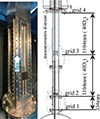 |
Fig. 1. Schematic representation and illustration of the CALIFS 5x5 test section. Figure from [16]. |
| In the text | |
|
Fig. 2. Representation of the system and the boundary conditions. |
| In the text | |
|
Fig. 3. Geometric representation of the grid without mixing vanes, view from above. |
| In the text | |
|
Fig. 4. Geometric representation of the grid section with mixing vanes. |
| In the text | |
|
Fig. 5. Representation of the periodic mirroring boundary condition of the mixing vanes in CALIFS. |
| In the text | |
|
Fig. 6. Cross sectional view of the mesh inside a subchannel downstream of the spacer grid (a), inside a gap between two rods (b), inside a subchannel through dimples (c), around the central rod through springs (d). Front section view of the mesh through the grid, near the outlet of the grid (e). The volume cells are represented in grey and the surface cells are represented in blue. |
| In the text | |
|
Fig. 7. Plot of |
| In the text | |
|
Fig. 8.
|
| In the text | |
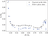 |
Fig. 9.
|
| In the text | |
|
Fig. 10. u+ = f(y+) for the fully developed turbulent flow in the gap between rods, z′=5 Dh upstream of the grid section. |
| In the text | |
|
Fig. 11. Vector representation of the non streamwise components of the averaged velocity field, at z′=5 Dh with mixing vanes. In the figure, the colour-map represents the scale of secondary flow velocity magnitude normalised by the bulk velocity. |
| In the text | |
|
Fig. 12. Plot of |
| In the text | |
|
Fig. 13. Plot of |
| In the text | |
|
Fig. 14. Plot of |
| In the text | |
|
Fig. 15. Plot of |
| In the text | |
|
Fig. 16. Plot of |Ux + Uy|/∥U∥, over the line (b) at z′=1 Dh (a), z′=10 Dh (b). |
| In the text | |
|
Fig. 17. Plot of I, over the line (b) at z′=1 Dh (a), z′=10 Dh (b). |
| In the text | |
|
Fig. 18. Plot of Lzz, over the line (b) at z′=1 Dh (a), z′=10 Dh (b). |
| In the text | |
|
Fig. 19. Plot of τ, over the line (b) at z′=1 Dh (a) z′=10 Dh (b). |
| In the text | |
|
Fig. 20. Barycentric map of componentality contours for a 5x5 bare rod bundle, DNS results from [22]. |
| In the text | |
|
Fig. 21. Anisotropy componentality contours at, z′=1 Dh (a), z′=5 Dh (b), z′=10 Dh (c), z′=15 Dh (d), in the case of the grid without mixing vanes and the chosen colour mapping (e). |
| In the text | |
|
Fig. 22. Reynolds stress tensor (a) and Anisotropy weight (b) plot over the subchannel line b from Figure 1 at z′=1 Dh. Reynolds stress tensor (c) and Anisotropy weight (d) plot over the subchannel line b from Figure 1 at z′=5 Dh. Reynolds stress tensor (e) and Anisotropy weight (f) plot over the subchannel line b from Figure 1 at z′=10 Dh. |
| In the text | |
|
Fig. 23. Anisotropy componentality contours at, z′=1 Dh (a), z′=5 Dh (b), z′=10 Dh (c), z′=15 Dh (d) and the chosen colour mapping (e). |
| In the text | |
|
Fig. 24. Reynolds stress tensor (a) and Anisotropy weight (b) plot over the subchannel line, z′=1 Dh in the case of the grid with mixing vanes. Reynolds stress tensor (c) and Anisotropy weight (d) plot over the subchannel line, z′=5 Dh in the case of the grid with mixing vanes. Reynolds stress tensor (e) and Anisotropy weight (f) plot over the subchannel line, z′=10 Dh in the case of the grid with mixing vanes. |
| In the text | |
Current usage metrics show cumulative count of Article Views (full-text article views including HTML views, PDF and ePub downloads, according to the available data) and Abstracts Views on Vision4Press platform.
Data correspond to usage on the plateform after 2015. The current usage metrics is available 48-96 hours after online publication and is updated daily on week days.
Initial download of the metrics may take a while.