| Issue |
EPJ Nuclear Sci. Technol.
Volume 6, 2020
|
|
|---|---|---|
| Article Number | 19 | |
| Number of page(s) | 22 | |
| DOI | https://doi.org/10.1051/epjn/2020007 | |
| Published online | 29 April 2020 | |
https://doi.org/10.1051/epjn/2020007
Regular Article
Validating nuclear data uncertainties obtained from a statistical analysis of experimental data with the “Physical Uncertainty Bounds” method
Los Alamos National Laboratory,
P.O. Box 1663, MS-P365,
Los Alamos,
NM
87545,
USA
* e-mail: This email address is being protected from spambots. You need JavaScript enabled to view it.
Received:
19
July
2019
Received in final form:
25
January
2020
Accepted:
12
February
2020
Published online: 29 April 2020
Abstract
Concerns within the nuclear data community led to substantial increases of Neutron Data Standards (NDS) uncertainties from its previous to the current version. For example, those associated with the NDS reference cross section 239Pu(n,f) increased from 0.6–1.6% to 1.3–1.7% from 0.1–20 MeV. These cross sections, among others, were adopted, e.g., by ENDF/B-VII.1 (previous NDS) and ENDF/B-VIII.0 (current NDS). There has been a strong desire to be able to validate these increases based on objective criteria given their impact on our understanding of various application uncertainties. Here, the “Physical Uncertainty Bounds” method (PUBs) by Vaughan et al. is applied to validate evaluated uncertainties obtained by a statistical analysis of experimental data. We investigate with PUBs whether ENDF/B-VII.1 or ENDF/B-VIII.0 239Pu(n,f) cross-section uncertainties are more realistic given the information content used for the actual evaluation. It is shown that the associated conservative (1.5–1.8%) and minimal realistic (1.1–1.3%) uncertainty bounds obtained by PUBs enclose ENDF/B-VIII.0 uncertainties and indicate that ENDF/B-VII.1 uncertainties are underestimated.
© D. Neudecker et al., published by EDP Sciences, 2020
 This is an Open Access article distributed under the terms of the Creative Commons Attribution License (https://creativecommons.org/licenses/by/4.0), which permits unrestricted use, distribution, and reproduction in any medium, provided the original work is properly cited.
1 Introduction
Nuclear data libraries such as ENDF/B-VIII.0 in the U.S. [1], JEFF-3.3 in Europe [2] or JENDL-4.0 in Japan [3] provide evaluated data mean values and associated uncertainties for nuclear data application calculations. The latter can be used to calculate performance and safety margins of application quantities due to nuclear data uncertainties. The reliability of these predicted margins critically depends on how realistic the underlying nuclear data uncertainties are and can impact policy and decisions that affect human welfare and economic considerations. Hence, it is important to be able to validate nuclear data uncertainties.
While validation of mean values is a well-established practice in the field of nuclear data evaluation, validation of all associated uncertainties is not routinely undertaken before releasing a new library. Methods exist, and are usually applied, that verify whether an evaluated covariance matrix is positive semi-definite or obeys sum-rules imposed on specific observable covariances [4]. While these methods provide necessary verification, they do not test whether an evaluated uncertainty is of a reasonable size given the input used to calculate it. One might argue that an evaluated uncertainty is not a physical quantity and there is no notion of right or wrong that can be validated. However, there clearly are uncertainty values that are unrealistically high or low for an observables given its physics information content coming from experimental data and theory at a specific point in time. For instance, given the accuracy of 252Cf(sf) total average neutron multiplicity experimental data, an uncertainty of 0.001% or 10% would be easily identified as unrealistically low or high. In this paper, we present one method by which one can estimate tighter, reasonable, bounds of a “quantity of interest” (QoI), for instance the 252Cf(sf) total average neutron multiplicity, that allow us to validate whether evaluated uncertainties are realistic.
To this end, we apply the “Physical Uncertainty Bounds” (PUBs) method [5] to more transparently validate whether evaluated uncertainties obtained from a statistical analysis of experimental data are within a realistic range. This method was developed by Vaughan et al. to assess physical bounds on the uncertainties of integrated systems or observables due to the limited fidelity of the governing physics sub-processes needed to simulate the system or observable. It was applied to many physics areas including plasma fusion reactions, material damage or material strength. Here, it will be applied to estimate conservative and minimal realistic uncertainty bounds on a nuclear data evaluation quantity obtained by a statistical analysis of experimental data given the information on all measurements used for the evaluation. Towards this goal, conservative and minimal realistic uncertainties are estimated for the sub-processes governing the nuclear data measurements such as, e.g., neutron attenuation or background scattering. This process of partitioning the uncertainties according to sub-processes is likely familiar to evaluators from the construction of covariances for individual experimental data sets, see e.g., [6–14]. It will be explained that we use the same experimental information compared to these methods but utilize the information from all measurements at once to bound a sub-process rather than informing the covariances of a single experimental data set. We apply the PUBs method to a test-case, namely, to estimate conservative and minimal realistic bounds of the neutron-induced 239Pu fission cross section, 239Pu(n,f), given the information content in its evaluation.
1.1 239Pu(n,f) cross sections released by the Neutron Data Standards
The evaluated 239Pu(n,f) cross sections and covariances we study here were released as a reference by the IAEA co-ordinated Neutron Data Standards (NDS) project [15].The evaluation is primarily based on a statistical analysis of many high-fidelity measurements, including multiple reactions, for instance, 6Li(n,t), 10 B(n,α), 235,238U(n,f) and 239Pu(n,f) cross sections and ratios thereof. The evaluation is performed via the code and database GMA [6,7] based on a generalized-least-squares algorithm.
Many NDS-evaluated uncertainties were significantly increased from the previous [16] to the current NDS release [15]. For instance, the current NDS 239Pu(n,f) cross-section uncertainties range from 1.3–1.7% compared to 0.6–1.6% for the previous one in the energy range of 0.1–20 MeV as can be seen in Figure 1. This increase was in answer to concerns within the community that the previous uncertainties may be unrealistically low given the experimental information entering the evaluation. It was assumed that they are underestimated due to (a) missing correlations between uncertainties of different experiments, (b) missing uncertainties of single experiments and (c) a missing systematic uncertainty component underlying many measurements using the same techniques. It was shown in reference [17] that indeed uncertainties of single experiments and correlations between uncertainties of different experiments were missing in experimental covariances related to the 239Pu(n,f) cross section in the GMA database. The original GMA output for the current NDS version provided similar evaluated uncertainties to the previous one as these concerns could not be addressed within GMA in a timely manner. However, an additional uncertainty component, namely the “unrecognized source of uncertainty” (USU) one estimated by a method proposed byGai [15,18,19], was added in quadrature to the GMA evaluated uncertainties. These increased uncertainties were then released as part of the current NDS data and covariances. However, these uncertainties were also questioned given that the USU method was not applied for NDS evaluations before and led to distinct changes in the covariances.
The previous and current versions of the 239Pu(n,f) NDS cross sections and covariances were adopted by ENDF/B-VII.1 [20] and ENDF/B-VIII.0 nuclear data libraries. Consequently, one may question whether the significantly different evaluated 239Pu(n,f) cross-section uncertainties in ENDF/B-VII.1 or ENDF/B-VIII.0 in Figure 1 are more realistic. Within this manuscript, the current NDS will be described as ENDF/B-VIII.0 and the previous one as ENDF/B-VII.1.
 |
Fig. 1 The ENDF/B-VII.1 239Pu(n,f) cross-section uncertainties (previous NDS) are compared to those of ENDF/B-VIII.0 (current NDS). |
1.2 Impact of ENDF/B-VII.1 and ENDF/B-VIII.0 239Pu(n,f) covariances on Jezebel
This particular example was also chosen because the distinctly different ENDF/B-VII.1 or ENDF/B-VIII.0 239Pu(n,f) cross-section covariances can lead to significantly different simulated bounds if they are used for integrated application simulations. To showcase this, the impact of different 239Pu nuclear data covariances on the Jezebel critical assembly was studied in reference [21]. Jezebel is a nearly spherical plutonium assembly with a minimally-reflected, metal core that consists to more than 94% of 239Pu. It has a fast spectrum, which is formally defined by the ICSBEP (International Handbook of Evaluated Criticality Safety Benchmark Experiments) handbook [22] as having more than 50% of the fissions occur at energies greater than 100 keV. In other words, the Jezebel critical assembly (PU-MET-FAST-001 in ICSBEP nomenclature) is sensitive to 239Pu(n,f) cross sections in the fast incident-neutron-energy range as can be seen in Figure 2. To be more specific, it is highly sensitive to the 239Pu(n,f) cross section and total average neutron multiplicity,  , in the energy range from 500 keV to 5 MeV, while the simulated keff is less sensitive to other cross sections (elastic, inelastic among them). When one folds these (n,f) sensitivities with ENDF/B-VII.1 and ENDF/B-VIII.0 239Pu(n,f) cross-section covariances following the sandwich rule, one obtains an uncertainty of 331 pcm and 903 pcm, respectively, in keff due to these covariances only [21]. These uncertainties are much larger than the benchmark keff uncertainty of 110 pcm reported in the most recent ICSBEP version of PU-MET-FAST-001. The difference in simulated keff uncertainty due to ENDF/B-VII.1 and ENDF/B-VIII.0 239Pu(n,f) cross-section covariances is also significant given that 270 pcm is the difference between a controlled and uncontrolled Pu-system at a certain point in criticality. ENDF/B-VII.1 related uncertainties are close to the 270-pcm limit, while those related to ENDF/B-VIII.0 indicate that the differential information on this reaction is not even close to be well-enough known to be within this critical limit. Hence, it is of interest for predicting realistic bounds of application quantities dependent on the 239Pu(n,f) cross section to validate which uncertainties, ENDF/B-VII.1 or ENDF/B-VIII.0, are more realistic.
An alternative method, compared to its evaluation procedure, should be applied to validate the 239Pu(n,f) cross-section uncertainties given that both ENDF/B-VII.1 and ENDF/B-VIII.0 239Pu(n,f) cross-section covariances are questioned. The PUBs method, described in detail in Section 2, is shown to be one possible method to undertake such a validation of evaluated covariances obtained by a statistical analysis of experimental data only. Section 3 demonstrates how it can be applied at the example of the ENDF/B-VII.1 and ENDF/B-VIII.0 239Pu(n,f) cross-section covariances. The resulting PUBs method estimated conservative and minimal realistic bounds indicate in Section 4 that ENDF/B-VIII.0 uncertainties are more realistic than ENDF/B-VII.1 given the information content used for the evaluation. The advantages and shortcomings of the PUBs method for the nuclear data field are also discussed in the same Section and compared to data reduction techniques [6,7,9–11] frequently used in the field of nuclear data evaluation. For instance, while the PUBs method is able to validate nuclear data uncertainties independently, its goal is not to provide evaluated nuclear datamean value like some of these evaluation methods do. Section 5 re-iterates the main results and conclusions, and ends with a short outlook.
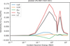 |
Fig. 2 The sensitivities of keff
of the Jezebel critical assembly [22] to the ENDF/B-VIII.0 239Pu elastic, inelastic, (n,f) cross sections, total average neutron multiplicity ( |

2 The Physical Uncertainty Bounds method
The PUBs method was developed at Los Alamos National Laboratory by Vaughan et al. [5] to assess physically informed bounds on uncertainties in integrated multi-physics systems or observables [5]. This methods deliberately forgoes quantifying uncertainties via only considering parametric uncertainty by varying parameters given a model. The parametric uncertainty approach can fall short by not considering correlation between parameters, and possibly spanning design/observable spaces that are unphysical, often resulting in improper bounds. Such methods also fail under extrapolation, in cases where there are large errors in themodel form. In order to overcome these limitations, the original PUBs method bounds uncertainties in physics processes using only experimental data, fundamental theory and numerical data obtained from first principles. Here, we will focus on using experimental information to inform the physics bounds. In addition, the method considers a set of curves spanning the function space between the bounds in order to address uncertainties due to model forms. These curves incorporate knowledge on the uncertainties and physics constraints on the functional dependencies of the observable on its sub-processes (e.g., monotonicity, convexity constraints) and are obtained without varying parameters of physics models.
The PUBs method as applied here can be summarized in the following steps:
- 1.
The QoI is parted into its constituting, independent, physics sub-processes. In this particular example, the sub-processes as presented in Section 3.2 (e.g., neutron attenuation, counts from impurities in the samples) are indeed independent of each other. If the assumption of independence does not hold, all of the correlated sub-processes would have to be considered together.
- 2.
An analysis is performed to determine the effects of variability in each sub-process on the eventual QoI. As part of this process, the dominant sub-processes causing the most variability on the QoI are identified (see Sect. 3.3). For instance, the QoI might have a negligible sensitivity to extreme variations of a particular sub-process. Hence, the bounds on this sub-process need not be quantified and the dimensionality of the problem can effectively be reduced.
- 3.
The bounds of variability for each sub-process are identified by using reliable experimental data, numerical data from first principles, or fundamental theory. If that cannot be established, the most extreme variability of the QoI stemming from the variability of the sub-process is quantified. If several measurements define the bounds of one sub-process, the combined bound given all experiments has to be established. This is discussed in detail for each sub-process in Section 3.4.
- 4.
The functional dependency of the QoI on each sub-process is also quantified (see Sect. 3.4). This functional form can be guided by physics constrains, experimental data and numerical data. An example for a physics constraints is, e.g., that a cross section above the unresolved resonance range is expected to be smooth.
- 5.
The last step in our analysis is not generally applicable for the PUBs methodology, since the assumption of independence among sub-processes does not always hold. However in this case, independence implies that a combined bound on the QoI can be supplied. As the QoI is parted such that all sub-processes are independent, the individual bounds of each sub-process are also independent. Consequently, the total bound of the QoI can be obtained in Section 3.5 by summing the bounds of each sub-process in quadrature.
It is shown in Section 3 how the PUBs method can be applied to estimate bounds on a nuclear data observable using the test case of the 239Pu(n,f) cross section. This example sets up a discussion in Section 4.3 how this methodology differs from other frequently used nuclear-data-evaluation algorithms or data-reduction formalisms [6,7,9–11,23].
3 Validating ENDF/B-VII.1 and ENDF/B-VIII.0 239Pu(n,f) cross-section uncertainties as an example for applying PUBs
3.1 How to validate ENDF/B-VII.1 and ENDF/B-VIII.0 239Pu(n,f) cross-section uncertainties
Here, we demonstrate the performance of the PUBs method using as a QoI a well-known example, namely, evaluated 239Pu(n,f) cross sections. More specifically, the PUBs method is used to investigate whether the significantly different ENDF/B-VII.1 or the ENDF/B-VIII.0 239Pu(n,f) cross-section uncertainties in Figure 1 are more realistic. The discussion focuses here on the energy range from 100 keV to 20 MeV.
If one wants to validate evaluated covariances with PUBs, the same input data (all measurements), information on measurement techniques and uncertainties as used for the evaluation of mean values and covariances should be used to correctly judge the information content available for the particular evaluations chosen for the QoI and, hence, the size of the standard deviation. As mentioned in the introduction, ENDF/B-VII.1 and ENDF/B-VIII.0 239Pu(n,f) cross sections and covariances were evaluated as part of the IAEA co-ordinated NDS project [15] based on a statistical analysis of experimental data using the code and database GMA [6,7]. Currently, there are 61 experimental data sets in the GMA database, where either the 239Pu(n,f) cross section is provided or where the 239Pu(n,f) cross section is given as a ratio to another reaction. These ratio data are given as ratios to either 6 Li(n,t), 10 B(n,α), 235 U(n,f), 238 U(n,γ) or 238U(n,f) cross sections. These data are used here as input for PUBs.
It is important to note for this validation that experiments providing fission cross sections do so by combining the results of multiple measurements and simulations, i.e., they are composite/integrated measurements. For instance, the fission detector counts charged particles; some counts may be due to fission fragments, and others due to background particles. The measured fission detector count rate is corrected for background counts by measurements or simulations as part of analyzing the fission cross section. In terms of the PUBs methodology, counting the charged particles with a fission detector and estimating the background are two separate sub-processes. There is a limit to how well we know each sub-process given pertinent experimental information on that sub-process across all measurements. For instance, a background uncertainty of below 0.2% uncertainty is difficult to achieve in a typical fission cross-section experiment due to limitations in background measurements and simulations. This 0.2% value is only the bound due to the limited knowledge on the background correction for one individual measurement. This uncertainty value would typically enter the uncertainty estimate for a total covariance matrix of one individual measurement that is then used as input for a generalized least squares analysis using, for instance, GMA. The PUBs method, however, requires to assess the total bound on the background estimation due to all measurements on the 239Pu(n,f) cross section. So, one has to consider how many different techniques are used to assess the background across all 61 measurements, and how will the total bound on the background reduce if the background is measured with these different, partially independent, techniques.
In estimating the bounds of the sub-processes we deviate slightly from the original formulation of the PUBs method in Section 2. In the third step, it is recommended to assess the physical bound for each sub-process. Here, two estimates are made: the first one is a conservative estimate of a sub-process given the experimental information across all measurements. The second estimate is a best-case, minimal realistic, one, to get a lower bound for each sub-process. These two bounds provide a realistic range of standard deviations given the combined knowledge for a specific sub-process.
These conservative and minimal realistic bounds on the sub-processes are then combined to a total conservative and minimal realistic bound on the 239Pu(n,f) cross section. The resulting two total bounds are used to assess whether ENDF/B-VII.1 or ENDF/B-VIII.0 239Pu(n,f) cross-section uncertainties are more realistic. If the total conservative bound, combined from all conservative sub-process uncertainties, falls below ENDF/B-VIII.0 standard deviations, the ENDF/B-VIII.0 ones are indicated to be unrealistically large. Similarly, if the total minimal realistic bound, is above the ENDF/B-VII.1 uncertainties, these are indicated to be unrealistically small.
One should note that for this analysis there is less emphasis on the functional dependence of the QoI on each sub-processes compared to the total bound sought. Also, throughout the whole manuscript, all uncertainties are understood to be 1-σ uncertainty values relative to the 239Pu(n,f) cross section(in %), unless otherwise noted, given that most experimental and the evaluated standard deviations investigated here are reported as 1-σ values.
3.2 Parting 239Pu(n,f) cross-section measurements into sub-processes
The QoI is evaluated based on experimental data only for the specific nuclear data uncertainties investigated here. Hence, its sub-processes are defined based on those physics sub-processes encountered in typical measurement types of the QoI. Most of the 61 measurements related to the 239Pu(n,f) cross section in the GMA database can be parted into three classes of experiments, see, e.g., [6,7], which are illustrated in Figure 3. These are three distinct measurement types that are designed to infer the same quantity, namely, the 239Pu(n,f) cross section. We follow here the nomenclature of reference [17,24] regarding these measurement types and summarize them briefly below, as applied to studying 239Pu(n,f) cross sections for energies from 100 keV to 20 MeV:
- (a)
In absolute measurements the (n,f) cross section, σ(E) (in barn), at energy, E, is determined via,
![Mathematical equation: \begin{equation*}\sigma(E) = \frac{(C_1-C_{b1})m\beta}{\phi N_1\varepsilon_1\tau_1}\left[1+\sum_i\sigma_{i1}N_{i1}\right]^{-1}, \end{equation*}](/articles/epjn/full_html/2020/01/epjn190048/epjn190048-eq2.png) (1)
(1)counting the count rate, C1, with the fission detector with detector efficiency, ε1, and deadtime, τ1. The total count rate, C1, has to be corrected for background particle counts, Cb1, mis-identified as fission counts, neutron attenuation and multiple scattering effects, β and m respectively. Neutron attenuation means in this context that neutrons are detected as part of the neutron flux ϕ but are then lost (attenuated) before they can lead to a fission event, i.e., reducing effectively C1. Multiple scattering effects lead to neutrons being detected at one energy for the neutron flux detection, losing part of their energy from the neutron flux to the fission detector and then leading to C1 induced by neutrons of lower energy than indicated by the neutron flux measurement. The number of 239Pu atoms in the sample, N1, needs to bedetermined along with the number of atoms in the sample of impurity i, Ni1, and their cross sections, σi1.
- (b)
In a clean ratio measurement, the QoI’s σ(E) is measured as a ratio to a reference observable with nuclear data representation σND2 (also in barn),
![Mathematical equation: \begin{equation*}\hskip-22pt \sigma(E) = \sigma_{\mathrm{ND}2}\frac{(C_1-C_{b1})N_2}{(C_2-C_{b2}) N_1}\delta\varepsilon_1\delta\tau_1\delta m\delta\beta\frac{\left[1+\sum_j\sigma_{j2}N_{i2}\right]}{\left[1+\sum_i\sigma_{i1}N_{i1}\right]}, \end{equation*}](/articles/epjn/full_html/2020/01/epjn190048/epjn190048-eq3.png) (2)
(2)measuring the count rates, C1 and C2, using samples with number of atoms in the samples, N1 and N2, in the same detector. Also, number of atoms in the sample, Nj2, for contaminating isotopes and their cross sections, σj2, need to be known for the sample of the reference measurement. The neutron flux nearly cancels out in this measurement type. Multiple scattering and attenuation effects, δm and δβ, are now quantified between the two samples, while background counts, C1b and C2b, need to be quantified for both measurements. The detector efficiency and dead time reduce to the difference in efficiency, δε1, and deadtime, δτ1, between measuring with samples 1 and 2.
- (c)
The indirect ratio measurement differs from the clean ratio measurement in as far as two different detector types are used to measure C1 and C2:
![Mathematical equation: \begin{equation*}\hskip-12pt \sigma(E) = \sigma_{\mathrm{ND}2}\frac{(C_1-C_{b1})N_2\varepsilon_2\tau_2}{(C_2-C_{b2}) N_1\varepsilon_1\tau_1}\delta m\delta\beta\frac{\left[1+\sum_j\sigma_{j2}N_{j2}\right]}{\left[1+\sum_i\sigma_{i1}N_{i1}\right]}. \end{equation*}](/articles/epjn/full_html/2020/01/epjn190048/epjn190048-eq4.png) (3)
(3)Therefore, the detector efficiency and deadtime, ε2 and τ2, need to be quantified Ifε2∕ε1 and τ2∕τ1 are written as δε1 and δτ1, one ends up with equation (2). Hence, the clean and indirect ratio measurements are treated as one type here, termed “ratio” measurements.
It should be clear from the discussion above that all experimental cross sections, σ(E), determined by equations (1)–(3) are integrated quantities. The constituting sub-processes are determined independently from each other either experimentally, by simulation or both, as follows:
- 1.
The number of atoms in the sample, N1, (for ratio measurements also N2) is usuallymeasured in measurements independent from counting C1 and C2.
- 2.
The neutron flux ϕ appearing in equation (1) is measured with a separate detector independent from the fission detector as depicted in the top panel of Figure 3. It does not appear in equations (2) and (3) it is replaced by determining instead
![Mathematical equation: $(C_2-C_{b2})m\beta\delta\tau\varepsilon_1/\left[\sigma_{\mathrm{ND}2}N_2\delta\varepsilon_1\tau_1 \delta m\delta\beta\left(1+\sum_j\sigma_{j2}N_{i2}\right)\right]$](/articles/epjn/full_html/2020/01/epjn190048/epjn190048-eq5.png) . Most of the variables in this term can be assigned to other sub-processes. Only the nuclear data of the reference cross section, σND2, remains which is, henceforth, assumed to be part of the neutron flux sub-process as these data are used to determine the neutron flux. This particular cross section is not used for defining other sub-processes unless the reference reaction appears as an impurity in the main sample with number of atoms
N1. Such a contamination was not listed for any of the measurements studied here.
. Most of the variables in this term can be assigned to other sub-processes. Only the nuclear data of the reference cross section, σND2, remains which is, henceforth, assumed to be part of the neutron flux sub-process as these data are used to determine the neutron flux. This particular cross section is not used for defining other sub-processes unless the reference reaction appears as an impurity in the main sample with number of atoms
N1. Such a contamination was not listed for any of the measurements studied here. - 3.
The detector efficiencies, ε1, δε or ε2, are either defined by measurements or simulations. The latter are based on data (e.g., stopping power data, angular distribution of fission fragments) independent from data of any other sub-process.
- 4.
The attenuation and multiple scattering effect are merged into one common sub-process, η = mβ for absolute and δη = δmδβ for ratio measurement, given that they are usually simulated with the same codes and underlying nuclear data.
- 5.
The background counts, Cb1 and Cb2, are often measured in dedicated experiments or simulated with nuclear data only weakly correlated with data used for simulating η and δη or correcting for impurities in the samples.
- 6.
The energy E of neutrons inducing the (n,f) cross section is also determined by measurement and a set of simple physics equations.
- 7.
The impurity correction factor,
![Mathematical equation: $\zeta = \left[1+\sum_i\sigma_{i1}N_{i1}\right]^{-1}$](/articles/epjn/full_html/2020/01/epjn190048/epjn190048-eq6.png) and δζ = [1 + ∑jσj2Nj2]∕
and δζ = [1 + ∑jσj2Nj2]∕
![Mathematical equation: $\left[1+\sum_i\sigma_{i1}N_{i1}\right]$](/articles/epjn/full_html/2020/01/epjn190048/epjn190048-eq7.png) , depends on impurities measured in the sample and the nuclear data for the impurities.
, depends on impurities measured in the sample and the nuclear data for the impurities. - 8.
The deadtime τ1 and δτ are corrected by calculations.
- 9.
The count rates C1 and C2 are determined based on a statistical counting process using detectors with efficiencies which are determined in a separate sub-process.
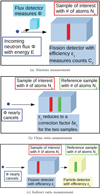 |
Fig. 3 Typical measurement techniques for absolute (upper panel), clean (middle panel) and indirect ratio (lower panel) measurements are schematically shown. |
3.3 Establishing dominant sub-processes
The sub-processes are listed in Section 3.2 according to how much variability they cause on the QoI. The lower the number is the higher uncertainties the particular sub-process will contribute to the total bound on σ(E). For instance, determining N1, the neutron flux, detector efficiencies, η/δη and the background are key elements for a fission cross-section measurement and can lead to large uncertainties on individual measurements [24] if not controlled, measured or corrected accurately. On the other hand, the impurity corrections, ζ and δζ, in 239Pu(n,f) cross-section experiments can be reduced to a negligible extent by using high-purity samples as for instance done in references [25,28,29]. As the correction is negligible, so is its bound resulting on σ(E).
3.4 Defining bounds and function forms for sub-processes
Minimal realistic and conservative 1-σ uncertainty bounds, Δxo and Δxc, are estimated in this sub-section for all sub-processes, x = {C1,2, N1,2, ϕ, …}, listed in Section 3.2. These two bounds are estimated as follows:
-
It is assessed how many different techniques i were used to determine the effect of the sub-process on σ(E) using information assembled in Table 1. For instance: how many different ways was N1 measured?
-
Minimal realistic and conservative 1-σ bounds,
 and
and  , on each technique i
to determine the sub-process are assessed. Information on the typical range of uncertainties for
, on each technique i
to determine the sub-process are assessed. Information on the typical range of uncertainties for
 and
and  for one measurement is taken from reference [24] or from the literature of particular experiments. It should be stressed that we depart here from the original PUBs philosophy. We do not take the most extreme value of uncertainty as proposed in the original formulation of PUBs but rather a conservative and a minimal realistic estimate of the uncertainty across many measurements using the technique
i. The reasoning behind this is that one can always have an unfavorable experimental condition that the uncertainty is high for one experiment on a specific xi
but by measuring the same xi
within multiple measurements using the same technique, one shrinks down to a realistic bound on
xi. Hence,
for one measurement is taken from reference [24] or from the literature of particular experiments. It should be stressed that we depart here from the original PUBs philosophy. We do not take the most extreme value of uncertainty as proposed in the original formulation of PUBs but rather a conservative and a minimal realistic estimate of the uncertainty across many measurements using the technique
i. The reasoning behind this is that one can always have an unfavorable experimental condition that the uncertainty is high for one experiment on a specific xi
but by measuring the same xi
within multiple measurements using the same technique, one shrinks down to a realistic bound on
xi. Hence,  and
and  are the combined bounds on a sub-process measured with one technique i
across many measurements using i, i.e., the limit of precision of this technique.
are the combined bounds on a sub-process measured with one technique i
across many measurements using i, i.e., the limit of precision of this technique. -
The total bounds, Δxo and Δxc on sub-process x are determined by:
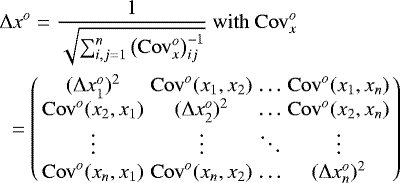 (4)
(4)and
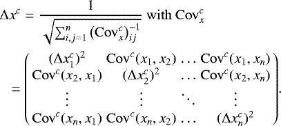 (5)
(5)The covariances, Covo(xi, xj) and Covc(xi, xj), between measuring the sub-process x with methods i and j are assessed based on expert judgment. Again, a conservative and minimal realistic estimate is given for these covariances to estimate Δxc and Δxo for sub-process x.
The functional forms of the QoI on each sub-process are defined based on the physics constituting the sub-process.
The techniques to determine N1, N2, ϕ, ε1, δε, η, δη, Cb1, Cb2, E, ζ and δζ for 239Pu(n,f) cross-section measurements in GMA [6] are listed. The measured observable, citation and GMA number are also given. The data sets providing data only below 100 keV are marked in yellow. The variables and acronyms are described in Tables 3 and 4.
3.4.1 Sub-process: determining N1 and N2
The number of atoms in the sample of the isotope of interest, N1, and of the reference sample, N2, enter as multiplicative, energy-independent, values in equations (1) and (2). Hence, an uncertainty on N1 and N2 leads to an uncertainty on the normalization of the 239Pu(n,f) cross section which is encoded in a fully correlated covariance matrix for the sub-process N1 and N2. More explicitly, the cross section is a linear function of 1∕N1 and N2∕N1.
As uncertainty in N1 and N2 leads to a normalization uncertainty, this uncertainty only applies to absolute 239Pu(n,f) data while it does not appear for shape data. Twenty-seven 239Pu(n,f) cross-section data sets are treated as shape data and, thus, do not provide any input on bounding N1 or N1 ∕N2. Out of the remaining 34 data sets, one [36] provides only experimental information below 100 keV. The variable N1 is quantified in 16 data sets, while N1∕N2 is quantifiedin 17 data sets as these are ratio measurements.
The variables N1 or N1 ∕N2 are often determined via α-counting measurements (α-count.)1 [25,29–33,37–39,43,45,46,49,50,53,60,61,63] independent from fission counting measurements as can be seen in Table 1. A 1% value is assumed as a conservative bound  across all measurements using α-counting to determine N1 in 239Pu samples following the literature of individual measurements and reference [24]. All but one measurement quantifying N1 ∕N2 are ratio measurements relative to 235 U. A slightly higher conservative bound
  % is assumed to measure the number of atoms in a 235U sample given the lower α-activity of 235 U. Non-zero correlations between the measurement uncertainties of N1 and N2 arise because both are measured with the same technique. These correlations need to be considered when estimating the total bound on N1 ∕N2, namely2:
 (6)
(6)
A value of 0.6 is assumed for cor(N1, N2) as, despite the measurement methods for N1 and N2 being the same, different isotopes with different α-activities are observed. The α-counting is sometimes paired with coulometric assay (coul. assay) [29–31,50], isotope de-composition [49] or destructive analysis (destr. anal.) [33] to determine contaminations in the sample. The associated bounds are accounted for in the sample impurity uncertainty, Δζ.
Apart from α-counting, direct weighting techniques [29,38,50,60]—two of them use micro-balances (micro-bal. weigh.) [32,60]—and measurements relative to thermal [28,32,41,43,45,52,60] were employed to determine either N1 or N1 ∕N2. Weighing techniques were always used to validate N1 or N1∕N2 obtained by α-counting. Due to this, the bounds associated with using this technique are assumed to be accounted for in the bound for measurements using α-counting. It is interesting to note that measurements of N1 or N1∕N2 using both, α-counting and weighing, techniques have total normalization uncertainties higher than 1.0% in the GMA database. The uncertainty for measurements relative to the thermal 239Pu(n,f) cross section, Δ(N3), assumes values between 0.6% and 1.7% across measurements employing this technique. This technique is often used as an auxiliary technique to validate α-counting results, but was also used on its own for few measurements as a ratio to the 235 U(n,f) cross section [1,28,41,52]. A value of 1.1% is assumed here as a total conservative bound. The threshold method (threshold meth.) [59] was only applied once to determine N1∕N2. It is not considered in the present analysis as the uncertainty of this one measurement cannot be cross-compared to another 239Pu(n,f) measurement.
The total conservative bound is estimated by using  , Δ(N1∕N2) and Δ(N3) for the standard deviations in equation (5). The correlation coefficient between
  and Δ(N1∕N2) is assumed to be 0.75 given that the same technique was used to determine both and one of two samples isotopes is the same. The correlation coefficient between
  and Δ(N1∕N2) and Δ(N3) is 0.5 which is probably high. The total conservative bound on ΔN comes out at 0.88%.
For the minimal realistic bound,  , Δ(N1∕N2) and Δ(N3) are assumed to be 0.9% each and the correlation coefficient between the former two and Δ(N3) is reduced to 0.3. The minimal realistic bound comes out to be 0.71%.
3.4.2 Sub-process: determining ϕ
The neutron flux ϕ has to be measured directly in measurements quantifying either the 239Pu(n,f) cross section or its shape. However, if the 239Pu(n,f) cross section is measured as a ratio to other observables, the neutron flux is indirectly determined through the ratio measurement. As mentioned in Section 3.2, the bounds of many sub-processes of this indirect measurement are determined separately but the nuclear data uncertainty of the reference observable remains. Most measurements of the current analysis are made as a ratio to the 235 U(n,f) cross section. A value of  % is used as a conservative bound for the 235U(n,f) cross-section nuclear data uncertainty based on the lower limit of ENDF/B-VIII.0 235 U(n,f) cross-section uncertainties. A value of
  0.6% is usedas a lower bound as this value approximates ENDF/B-VII.1 uncertainties.
The neutron flux is directly measured with the associated particle technique (ASSOP) [25,30,33,37], recoil particle measurements (REC) [31,33,38,56], relative to manganese baths (MANGB) [32,33] and with indirect Boron-pile measurements (ind. B-pile) [57]. Auxiliary calculations (calc.) [33] and measurements relative to various other reactions [56,60] were used in only a few cases. The neutron flux was determined once by an activation measurements (ACTIV) [61]. The manganese baths were mostly used jointly with the associated particle technique. Hence, a common bound for both is estimated. In recoil particle measurements used for this analysis, ϕ is directly measured with a recoil telescope proton counter. Four measurements [31,38,56] use this technique independently from associated particle measurements, but it is also often used jointly. A joint conservative bound Δϕ2 =0.8% over all techniques is used based on comparing uncertainties appearing for all three main techniques. A minimal realistic bound  =0.8% is used for the associated particle technique and
  % is used for measurements of the neutron flux using the recoil particle technique. The latter value is rather low compared to uncertainties in [31,38,56] related to determining ϕ via the recoil particle technique (larger equal than 1.7% in most cases). For Δϕc, it is assumed that the correlation between Δϕ1 and Δϕ2 is 0.2 given that the evaluated uncertainties of the 235U(n,f) cross section were partially obtained based on measurements using the associated particle technique, etc., to obtain ϕ. This leads to a conservative estimate on understanding ϕ in 239Pu(n,f) cross-section measurements of 0.74%. Zero correlation between Δϕ1, Δϕ2 and Δϕ3 is assumed to estimate Δϕo leading to Δϕo = 0.45%
Following the template in reference [24], it is assumed that the correlation matrix is constant with a correlation factor of 0.75.
3.4.3 Sub-process: determining ε1, ε2 or δε
The detector efficiency ε is an integrated correction in itself but the uncertainties are often reported in a combined manner. Thus the sub-processes contributing to ε are treated in a combined manner as well. The corrections entering the detector efficiency are [17,81]:
-
The stopping power (stopp. pow.) of the sample needs to be accounted for. Usually, this correction is calculated [29,36,37,45,49,50,60] using stopping power data which lead to strong cross-correlations across measurements correcting for this effect. The stopping power was measured in two cases [36,63].
-
The inherent fission fragment angular distribution (FF ∠) also needs to be corrected when assessing ε. This correction is usually calculated [25,31,33,37,59,60,63]. It was also measured in a few cases [45,60]. If it is calculated, recourse to the same or similar underlying data will be taken leading to a strong correlation of this correction across measurements.
-
The angular distribution of fission fragments induced by the kinetic forward boost (forw.-boost) of the fission fragments is usually corrected using kinematic calculations [29,45,59]. It was measured in only one case [39]. This correction is highly correlated between measurements as the same function is used for the correction across different measurements.
-
The sample thickness (thickn.) leads to a correction in ε that isoften calculated [25,31,39,46]. It was measured in only one measurement series [33]. This correction is highly correlated between measurements as the same input data are needed for the correction.
-
Target roughness (roughn.) is usually measured [33], e.g., via similar α-counting measurements (α-count.) [25] or α-spectroscopy (α-spectr.) [30,48,49]. It was calculated in only one case [38].
-
In a few cases, the detector design affected its efficiency leading to a geometrical correction factor (geom.) which is usually calculated [36] or Monte Carlo simulated [43,46]. Again, similar underlying nuclear data are used for calculating this correction factor leading to strong correlations between measurements for this uncertainty source.
A general, overarching, technique is named to determine ε for several measurements, namely, identification of particles through pulse-height discrimination (PHD) [28–31,36–39,43,45,46,49,50,52,57,59,61,65,67,70,71,75]; ε is calculated (calc.) [33,56,57,61,64,71,75], measured (meas.) [33,56,61,66,68,74,75], extrapolated (extrap.) [36,38,43] or measured with a rotated detector (rotat. det.) [38,39,50]. In a few cases, ε is calculated using an assumed prompt fission neutron spectrum (PFNS) [57], obtained by normalization (normal.) [71] or determined by a transmission measurement (transm.) [68] and pulse-shape discrimination (PSD) [70,74]. The correction ε can be reduced by the design of the fission chamber or selecting a thinness of samples to have maximal efficiency (Design) [65,79].
A base value of 1.2% for shape/absolute measurements of the 239Pu(n,f) cross section is assumed. Usually, the same or a very similar detector with similar corrections is used for ratio measurements as a ratio to 235 U(n,f). Some corrections of ε2 will be determined very similarly (kinematic forward-boost, geometry, roughness, thickness) while different data will be used for some others (inherent fission fragment distribution, stopping power) leading to assuming a non-zero correlation cor (ε1, ε2) = 0.6 between ε1 and ε2. The uncertainty on δε = ε1∕ε2 is calculated by:
 (7)
(7)
assuming that all uncertainties are given relative to ε1, ε2 and ε1 ∕ε2. When populating the covariance matrix in equation (5) with Δ(ε1) = 1.2%, Δ(ε1∕ε2) = 0.85% resulting from Equation (7) and a correlation coefficient of 0.9, one obtains a conservative bound of 0.77%. The base-value is reduced to 1.0% for the minimal realistic bound given that many measurement techniques are used to determine the detector efficiency leading to Δεo= 0.65%. The cross section is assumed to be linearly dependent on ε following reference [24].
3.4.4 Sub-process: determining η or δη
Multiple scattering and neutron attenuation effects are often reduced by setting the room up favorably (Room set-up) [31,39] or designing the measurement (design) [65,66] such that there is minimal scattering material in the surrounding of the measurement. The attenuation effect reduces in ratio measurements as one only corrects for neutronsattenuated (i.e., lost) between the two foils (Pu sample and ratio isotope sample). Also, multiple scattering effects reduce in ratio measurements as one has to only correct for the difference in the effect on the 239Pu(n,f) cross section and its reference counterpart. Hence, the total bound shrinks down to the combined bound of δη = δβδm of ratio measurements considering all techniques to determine δη.
Multiple scattering and attenuation effects are usually corrected via Monte Carlo calculations (MC) [25,32,33,41,46,48,53,56,57]. It is stated for many measurements [29–31,36–38,45,50,59,60,70,71,75] that these effects were “calculated”. It is assumed that all these calculations take recourse to the same or similar nuclear data leading to strong correlations between δη uncertainties across many measurements. Even though, these measurements did their own correction of δη, the uncertainty will shrink down to the common underlying uncertainty due to nuclear data and code uncertainties. δη was directly measured in a few measurements [33,36–38,45,71,80], for instance, by rotating the detector (rotat. det.) [39,50]. This second class of determining δη leads to a reduction of the overall bound.
The bounds due to multiple scattering, Δm, and attenuation, Δβ, have to be considered to determine a bound on η or δη. There is a non-zero covariance Cov(m, β) between the multiple scattering and attenuation correction given that the same or similar underlying nuclear data are usually used to correct both. Hence, Cov(η) reads3 :
 (8)
(8)
The term Cov(βi, βj) is estimatedbased on reference [24] to be 0.2% up to 200 keV linearly decreasing to 0.02% at 20 MeV. This estimate is based on the typical range of attenuation uncertainties in a ratio measurement. The term Cov (mi, mj) is estimated by assuming that Δ(δm) shrinks down to 0.3% across ratio measurements. A Gaussian correlation matrix is used to estimate the correlation coefficients,
![Mathematical equation: \begin{equation*}\mathrm{Cor}_{i,j}= \exp\left\{-\left[(E_i-E_j)/\mathrm{max}(E_i,E_j)\right]^2\right\}, \end{equation*}](/articles/epjn/full_html/2020/01/epjn190048/epjn190048-eq29.png) (9)
(9)
for all covariances appearing on the right-hand side of equation (8). This estimate is based on the assumption that nuclear data uncertainties are usually more strongly correlated for energy bins close to each other than far apart. This correlation matrix is used as an approximation for possible functional dependencies of the cross section on η which can be obtained by sampling from Cov(ηi, ηj). The “true” functional dependence of the cross section on η is unknown as it would need to be quantified considering a complex interplay of nuclear data and codes used for determining η across all relevant measurements.
The conservative bound Δηc shown in Figure 4 is quantified following equation (8). The minimal realistic bound Δηo is obtained by dividing Δηc through  taking into account that measurements of multiple scattering and attenuation corrections supply an independent quantification of η.
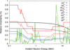 |
Fig. 4 The conservative and minimal realistic bounds are shown for the sub-processes η, E, Cb and C (multiple scattering and attenuation, incident neutron energy, background and counting rates, respectively). |
3.4.5 Sub-process: determining Cb1 and Cb2
Similarly to δη and η, the background corrections Cb1 and Cb2 can be reduced by setting the room up accordingly [31,32], by using a shadow-cone (shadow-cone) [31], by careful detector design (det. design) [33,38], by using shielding (Shielding) [28], by using clearing magnets (clear. magnet) [59] and by design of the measurement at large (design) [60,67,80]. The remaining background is often measured [25,29,32,33,36,38,41,43,45,46,49,51,52,56,57,60,61,63,65,66,68,79,80]. Some of these measurements are with sample out (Sample out) [43,49,71,75], use various monochromatic filters (monomchrom. filt.) [51], are time-of-flight measurements (TOF) [37,61] or use the black resonance filter technique (BRF) [51–53,56,57,66,68,69,71,74,75,78,79]. The background corrections, Cb1 and Cb2, are also identified by pulse-height discrimination (PHD) [30,36–39,43,45,46,48–50,52,59,61,65–67,70,75], calculated [36,60,68] (in some cases via Monte Carlo simulation [33]) or estimated by fitting a curve to measured data (fit) [41,57]. The background is also identified by pulse-shape discrimination (PSD) in two measurements below 100 keV [70,74].
The background uncertainty of data set [41] is used as a baseline uncertainty for  with the assumption that the uncertainty does not fall below 0.22% across all measurements. This lower limits follows reference [24] which statesthat a background uncertainty of 0.2–0.3% is technically achievable in a single measurement. It is assumed for the minimalrealistic estimate that there are three different completely independent background determination techniques (measurement, calculation, PHD) with an independent underlying uncertainties of the same values as
  . Hence,
  as shown in Figure 4. Possible functional dependencies of the cross section on Cb are encoded in a correlation matrix defined in equation (9). This correlation shape was used as nuclear data covariances underlying the calculated background correction are often strongly correlated near the diagonal and less strongly correlated for energies far apart. The same behavior is expected if uncertainties are stemming from parameter uncertainties related to fits of measured background.
3.4.6 Sub-process: determining E
Energy uncertainties are often given relative to E or as time resolution which are then converted into uncertainties relative to cross section. An energy uncertainty of 1% relative to energy is used here as a base-line uncertainty given that this value was frequently used in the GMA database if no values for ΔE were provided in the literature of a particular measurement. The conservative and minimal realistic estimate are then based on this baseline considering a reduction of uncertainties because different independent techniques were used to determine the energy E.
The energy was determined for 239Pu(n,f) cross-sectionmeasurements in the GMA database by the associated particle technique [25,30], recoil particle measurement [29,31,38,45,50] and time-of-flight determination (TOF) [28,33,37,41,48,49,52,53,56,57,59,65,66,68–71,73–75]. A larger sub-set of measurements was also undertaken using mono-energetic neutron sources (mono-E) [29,31,39,43,45,46,50,61–64,80]. In only few measurements, a manganese bath [32,36], spectrum correction (spectr. cor.) [32], an oil bath [36], indirect Boron pile measurements [36], α-monitors (α-monitor) [39,53], monochromatic filters [51], stacked target irradiation (STTA) [56], coincidence measurements (COINC) [56], silicon surface barrier detector measurement (SSBD) [60], method of slowing-down-time in lead cube (SLODT) [67,79], methods using scandium, iron and silicon filters (FNB) [51] and using unspecified filters [78] were used to determine E. The energy was calculated in a few cases [43,61].
It was assumed that two of these techniques are completely independent for estimating ΔEc, while four independent techniques were assumed to estimate ΔEo. One might argue that the number of independent techniques is higher. However, several techniques were used for identifying E in the same measurements leading to cross-correlations.
The energy uncertainty relative to the fission cross section depends on the partial derivative of it with respect to energy. Hence, in energy ranges where the 239Pu(n,f) cross section is smooth, the uncertainty contribution is small. However, in energy ranges, where the cross section has a large slope, e.g., at a multiple-chance-fission threshold, the contribution of ΔE to the total bound can be significant as can be seen in Figure 4.
The correlation matrix encoding the functional form of E is obtained in cross-section space by assuming that ΔE is fully correlated in energy space and then transforming to cross-section space via partial derivatives.
3.4.7 Sub-process: determining ζ or δζ
The uncertainty on 239Pu(n,f) cross sections due to contaminations in the samples can be effectively controlled by having samples of high purity rendering the correction factor negligibly small. For instance, the measurements [25,28,29,32,36,43,50,52,61,68] used 239Pu samples of a purity of larger than 99.9%. The corrections ζ and δζ are small for these measurements reducing the total bounds on this sub-process significantly.
Two uncertainty sources contribute to the total bounds of ζ: One is the nuclear data uncertainty of the fission cross section of the contaminant. The second part is due to the measurement of the level of contamination. These contaminations are mostly measured via α-counting [29,33,36–38,43,45,46,48–50,52,60,61,63] and spectral analysis (Spectr. anal.) [32,38,48,53,60,63,79]. Other techniques were employed for a few measurements, namely: residue weighing (Resid.-weigh.) [31], measurements with high-purity germanium detectors (meas. (HPGE)) [41], destructive analysis [43], measurements relative to the thermal (n,f) cross section [43], direct weighing [52], resonance measurement (reson. meas.) [71] or the corrections ζ were calculated [71]. A total bound of  0.1% and δζo =0.05% for determining contaminants in Pu samples and
  =0.2% and δζo=0.1% for contaminants in U samples are estimated based on reference [24]. The bound on U samples is higher given that fewer measurements in the database [28,45,52,59,63] had U samples of purity higher than 99.9%. A bound on ratio measurements Δ(δζ) is determined by using
  leading to
  =0.15% and
 =0.07%. A relatively high correlation factor between δζ1 and δζ2 is assumed as the same measurements were used to determine the contaminations. The total bound is obtained by populating covariances in equations (4) and (5) with
  ,
,  and correlations between those two values of 0.8 leading to a small Δζc = 0.09% and Δζo = 0.05%. The functional dependence of the cross section on ζ is approximated by a linear function (full correlation) given that the measurements of the contamination level is the same for all E. The nuclear data covariances of the contaminating isotope are usually not fully correlated. However, the level of contamination contributes usually to a larger extent to Δζ compared to the nuclear data uncertainties.
3.4.8 Sub-process: determining τ or δτ
Deadtime could affect past measurements significantly due to α pile-up such that corrections were needed. However, it can be very well controlled to make it a negligible uncertainty source in today’s measurements. A bound has to be quantified separately for absolute and ratio measurements as τ is not necessarily the same for a 239Pu samples versus, e.g., a 235U sample due to the larger α-activity of the former. Deadtime is caused by the finite response of the drift gas in the detector, data-acquisition and cables. The latter two sources of uncertainties can be assumed to be fully correlated between the 239Pu(n,f) cross-section and the ratio measurement as the same types of cables, data acquisition, etc., are usually used in the same measurements. The drift gas response is not the same for 239Pu versus the ratio sample given the different α-activity. The bound uncertainty on δτ can be calculated via4
 (10)
(10)
The values τ1=0.2%, τ2 =0.15% and cor (Δτ1, Δτ2)=0.75 are used to obtain a conservative estimate for  , while τ1=0.1%, τ2 =0.05% and cor (Δτ1, Δτ2)=0.75 are used for
  .
.
The covariance matrix in equation (5) is populated with  =0.13% and δτ1 =0.2% and a correlation factor of 0.9 to get a total conservative bound yielding Δτc =0.11%. The minimal realistic bound Δτo=0.07 is obtained by
  =0.07% and δτ1=0.1% and a correlation factor of 0.8. It is stated in reference [24] that the shape of the deadtime is usually well-known and the uncertainty is on its normalization leading to a fully correlated covariance matrix for δτ.
3.4.9 Sub-process: determining C1 and C2
The uncertainty on C1 and C2 is a counting uncertainty independent from one measurement to another as well as one E to another. It could be reduced to zero if one could count infinitely long. However, one cannot count infinitely long, even if one adds up the counts of all measurements. Hence, a small non-zero bound remains that is negligible compared to other bounds. The bounds ΔC1 are estimated by using the statistical uncertainties ΔCT of [41]. This particular measurement was used as it is covers the full energy range investigated. It is assumed for the conservative bound that there are about 10 measurements in each energy bin covering the energy range investigated here if one uses all data sets in the GMA database. The energy bins are assumed to be broader for the minimal realistic bound, so that one has 15 measurements in each bin. Hence,  and
and  . The contribution is negligibly small as can be seen in Figure 4. The independence of C from one E to another is encoded in a diagonal covariance matrix.
3.5 Total bounds on the 239Pu(n,f) cross section
A total conservative and minimal realistic bound can be calculated by summing the covariances of each sub-process xk in quadrature
 (11)
(11)
as the sub-processes were selected such that they are independent from each other. The uncertainty range of all bounds is summarized in Table 2 to compare the different level of uncertainty for each sub-process. When one takes the square-root of the diagonal, the conservative and minimal realistic bounds in Figure 5 are obtained. The conservative and minimal realistic bounds enclose ENDF/B-VIII.0 239Pu(n,f) uncertainties while ENDF/B-VII.1 uncertainties lie below the minimal realistic bound. The correlation matrices obtained for the conservative and minimal realistic bound in Figure 6 using the covariances associated with the sub-processes are strongly correlated. These shapes are more similar to ENDF/B-VIII.0 than ENDF/B-VII.1 covariances (Fig. 6) in the relevant energy range. However, the assumptions on the functional dependence of the cross section on the sub-processes are not as well informed as those on the total bounds. Hence, no strong conclusion should be drawn regarding the validity of correlation matrices for 239Pu(n,f) cross sections in ENDF/B-VIII.0 and ENDF/B-VII.1.
The conservative and minimal realistic one-sigma bounds relative to the 239Pu(n,f) cross-section for each sub-process are summarized. If these uncertainties vary in size with incident neutron energy, their range is provided andshown explicitly in Figure 4. Also, functional forms are briefly summarized. The variables listed are defined in Table 3.
Variables frequently appearing throughout this manuscript are listed in order of their appearance.
Acronyms frequently appearing throughout this manuscript are listed in order of their appearance.
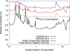 |
Fig. 5 The conservative and minimal realistic total PUBs bounds are compared to ENDF/B-VII.1 (previous NDS) and ENDF/B-VIII.0 (current NDS) 239Pu(n,f) cross-section uncertainties. |
 |
Fig. 6 Correlation matrices obtained for the conservative and minimal realistic PUBs bounds are compared to correlation matrices associated with ENDF/B-VII.1 and ENDF/B-VIII.0 239Pu(n,f) cross sections. |
4 Results and discussion
4.1 Results
The total conservative and minimal realistic PUBs bounds in Figure 5 indicate that the ENDF/B-VIII.0 239Pu(n,f) cross-section uncertainties are more realistic than their ENDF/B-VII.1 counter-parts. It was assumed that uncertainties of single 239Pu(n,f) cross-section experimental data sets in GMA are either missing or unrealistically low. It was also assumed that correlations between uncertainties of different experiments are missing or underestimated. It is explicitly shown in reference [17] that this is indeed the case and affects the uncertainty information of many 239Pu(n,f) cross-section measurements in GMA. This study focuses on a detailed uncertainty analysis of individual measurements in GMA. It will be explained in Section 4.3 that while the same input information is used for both studies, that some aspects of the PUBs formalism to obtain total bounds differ from how the evaluated covariances are obtained with GMA. Hence, PUBs indicating that ENDF/B-VII.1 239Pu(n,f) cross-section uncertainties are underestimated is not only well-supported by USU studies [15,18,19], but also by looking explicitly at the covariance input for the evaluation.
The minimal realistic and conservative uncertainties could be reduced by considering information from a new type of measurement that reduces the bounds on one or several sub-processes drastically. It would be favorable if multiple experiments use this technique to guarantee that the new measurement type is sufficiently validated. PUBs results can guide experimentalists in what sub-process should be tackled by these new measurements to enhance our understanding of the QoI; they provide an importance ordering of the sub-processes according to how much variability/ uncertainty each of them causes on the QoI. In the current analysis, it is evident from Table 2 that the uncertainties in determining the numbers of atoms in the sample, the neutron flux and the detector efficiency contribute substantially to the total bound on the 239Pu(n,f) cross section. Addressing these sub-processes in a targeted measurement could reduce the total bounds on the 239Pu(n,f) cross section. It should be noted that Δϕ contains substantial uncertainties of the evaluated 235U(n,f) cross section. Hence, a high-precision 235U(n,f) cross-section measurement has the potential to reduce bounds on the 239Pu(n,f) cross section if this measurement is included in an evaluation.
One caveat of the current analysis is that it provides conservative and minimal realistic bounds given present-day knowledge. If a new experiment uncovers a previously unknown sub-process that should have been corrected in all other past measurement, this effect will lead to a missing common systematic uncertainty across all measurements. This uncertainty would also be missing in the current PUBs estimate. The USU technique described in reference [15,18,19] might be able to capture this uncertainty if it leads to a spread across all measured data of about the size of the uncorrected effect. If this missing effect leads to an equal off-set in all data-sets, the USU technique will not capture it.
4.2 Discussion of deviations from original PUBs Formulation
It was suggested in the original PUBs method formulation that the most extreme bounds should be used for the estimate. Here, we deviate from the original formulation in as far as reasonable conservative and minimal realistic bound are estimated. The minimal realistic bound corresponds to a lower limit. It is assumed that it is difficult to determine a sub-process to an uncertainty level below this bound. The conservative bound is, as its name suggests, an upper bound on how well a sub-process is understood. Individual measurements might cite larger uncertainties for a particular measurement but it is realistic to assume that the combined knowledge across many measurements has uncertainties on this sub-process below this conservative bound. Hence, it is unlikely that ENDF/B-VII.1 239Pu(n,f) uncertainties are realistic given the current knowledge on the data in the GMA database.
4.3 Discussion of PUBs in comparison to other evaluation and data reduction procedures
It was shown that the PUBs methodology is an auxiliary technique that can be used to validate nuclear data uncertainties stemming from a statistical analysis of experimental data only. One might argue that some aspects of the PUBs method are not entirely new to the field of nuclear data evaluation. In order to draw out similarities and differences, we compare here to the GMA [6,7] and the AGS [9–11] data reduction and uncertainty quantification approaches. The GMA approach was chosen as it was used for NDS evaluations discussed here. AGS was chosen as its philosophy was implemented in many codes [12–14] and used for evaluation related efforts over decades, e.g., [87,88] for one evaluation in the mid-80s and another one in 2019. What is similar for all three approaches, GMA, AGS and PUBs, is that:
-
the different sub-processes, as described in Section 3, are identified for a specific measurement type, and,
-
that it uses information on individual experiments entering the evaluation such as compiled in Table 1, and
-
relies in some part on expert judgment.
The difference lies in how this information is used. GMA uses it to assign uncertainties relative to the QoI for a specific sub-process for each individual measurement in its input decks. For instance, uncertainties can be provided related to E, C, ϕ, etc., relative to σ. These uncertainties are either explicitly provided by the experimentalist or estimated based on expert knowledge and information such as compiled in Table 1. The AGS method goes a step further and starts from the raw data of an individual measurement to reconstruct σ and estimate covariances for these specific measurements along the way using knowledge about the data reduction scheme, measurement information, associated uncertainties and expert judgment to compensate missing facts. Both techniques also allow to estimate correlations between experiments. Here, however, the PUBs methodology takes “a view from above” instead of going into the uncertainty details of each individual measurement. It is assessed how well one can determine each sub-process, e.g., multiple scattering, detector efficiency, using information across all measurements for one single sub-process at a time. Expert judgment assumptions also enters estimating PUBs bounds, namely on: (1) what is the base-line uncertainty of one technique, (2) how many techniques are truly independent and (3) how is the functional dependence of the cross section on the sub-process approximated? These expert judgment assumptionswere informed by comparing uncertainties across different measurements and listing explicitly in Table 1 which techniques were used to determine each sub-process. Again, this kind of expert judgment and informing uncertainties of one measurement by similar ones, are approaches frequently used to generate input for GMA and AGS but the aim (informing individual experimental covariances versus the bounds of a sub-process) is different.
This difference in philosophy has important implications. As PUBs focuses on bounding individual sub-processes, this method cannot be used to provide evaluated mean values and covariances for nuclear data libraries as the former are not quantified within this technique. PUBs can yield several functional forms spanning the space between PUBs bounds. However, it provides no ordering of importance of one of these forms versus another, i.e., a designated mean value that should be used for simulations. However, many statistical techniques [6,7,9–14,23,82–84] exist to provide this information. However, PUBs provides more explicitly information on which sub-process is better or less well-known across all measurement as was for instance done in Table 2. This importance ordering can provide input on a possible focus of future measurements. It can be also extracted from AGS and GMA input by going through the uncertainties corresponding to a specific sub-process for all individual data sets and combining that information which follows the PUBs-philosophy. In addition to that, PUBs as applied here allows us to give a range of reasonable uncertainties, i.e., minimal realistic and conservative bounds that can help in validating existing uncertainties. PUBs also differs from nuclear data evaluations using models, such as, for instance, used and described in reference [23,89,90] in as far as it forgoes spanning a reasonable physics space for a QoI by varying parameters of a model.
All of these methods that are compared to above are usually more strongly associated with evaluating rather than validating uncertainties. PUBs, however, does not aim at evaluations as mentioned above but provides a sanity check on whether the evaluated uncertainties obtained are in a reasonable range given the expert knowledge on how well we truly understand the physics sub-processes contributing to the covariances on the observable of interest. This sanity check is frequently undertaken as part of approving covariances for inclusion in nuclear data libraries, but in an informal manner. For instance, it is frequently discussed at national or international nuclear data meetings that total evaluated standard deviations of a specific observable are unrealistic given that it depends on a specific sub-process that brings on its own a larger uncertainty than the evaluated ones. However, such discussions are anecdotal while the PUBs method, on the contrary, provides a formalized procedure putting this expert judgment estimates in a mathematical framework that enables giving concrete bounds. This framework uses, as highlighted above, procedures known from data reduction schemes to prepare the evaluation input.
It should be pointed out that the PUBs method was applied here to an observable where ample experimental information is available over the entire relevant incident neutron energy range to inform the PUBs bounds. The PUBs method can be also applied to observables with scarce experimental information. The physics bounds are then estimated through theoretical considerations or simulations. Typical information encoded in such physics bounds could be, for instance, that a (n,f) cross section is expected to be smooth above the resonance range and features, such as the sharp increase, of the cross section around the second-chance-fission threshold are expected to appear. Another way to quantify PUBs bounds based on theoretical considerations is using models which include physics laws as well as model approximations. The physics laws are expected to provide immutable constraints on the observable, while one has to assess the bounds on the QoI due to model approximations [85]. A PUBs bound can be also estimated, if experimental/simulated data exist to quantify bounds on only a limited part of a QoI, but, in addition to that, physics smoothness constraints apply to a larger part of the QoI – enclosing the part informed by experimental information. This combined information can then be used to bound the energy ranges without experimental/simulated data via interpolation and extrapolation obeying the physics smoothness constraints on the functional dependence of the QoI on its sub-processes.
5 Summary, conclusions and outlook
The Physical Uncertainty Boundary (PUBs) method developed at Los Alamos National Laboratory by Vaughan et al. [5] was shown to be a viable method to validate nuclear data uncertainties evaluated by experimental data only. This method differs from frequently-used nuclear data evaluation techniques and data reduction procedures, e.g., [6,7,9,10,23], in that it provides “a view from above” quantifying how well we truly understand each sub-process contributing to uncertainties on the quantity of interest (QoI). For instance, one of many possible sub-processes could be determining the number of atoms in the sample or the neutron flux. The PUBs method then quantifies how much uncertainty these sub-processes contribute to the one on the 239Pu(n,f) cross section. Hence, this method provides a mathematically formalized procedure to assess the bounds of each sub-process to then give a complete bound on the QoI. Some steps of this procedure – parting a QoI into sub-processes for uncertainty quantification and the physics input – are the same as for other techniques [6,7,9–14] but its output (how well-we understand each sub-process and obtaining conservative and minimal realistic bounds) is different. Thus, it does not provide mean values and, therefore, cannot be used to provide an evaluated data set for a nuclear data library. However, it provides an explicit importance ordering of all sub-processes and the means to validate evaluated uncertainties for a QoI.
Here, we used this method to estimate conservative and minimal realistic bounds on the 239Pu(n,f) cross-section uncertainties given the knowledge used for a specific evaluation. Here, we focus on those 239Pu(n,f) cross sections uncertainties in ENDF/B-VIII.0 and ENDF/B-VII.1. These data and covariances were supplied by the IAEA co-ordinated Neutron Data Standard project [15] based on a statistical analysis of mostly experimental information.These particular uncertainties were validated as an example given that they are so significantly different that this difference can potentially impact some application calculations. For instance, ENDF/B-VIII.0 239Pu(n,f) cross-section covariances nearly triple the simulated uncertainties on the criticality of the Jezebel critical assembly due to this cross section compared to using ENDF/B-VII.1 239Pu(n,f) cross-section covariances [21]. In addition to that, questions were raised concerning the validity of both bounds. ENDF/B-VII.1 uncertainties were assumed to be underestimated because of missing/underestimated uncertainties of single experimental data sets and missing/underestimated cross-correlations between uncertainties of different data sets [15]. An additional uncertainty–accounting for these missing uncertainties–was therefore added a-posteriori for ENDF/B-VIII.0 uncertainties based on the USU method [18]. The PUBs conservative and minimal realistic estimate in Figure 5 indicate that ENDF/B-VIII.0 239Pu(n,f) uncertainties are more realistic. Hence, uncertainties and correlations are probably missing in the database underlying the 239Pu(n,f) evaluation. These uncertainties should be updated for the next release of the 239Pu(n,f) cross section through the Neutron Data Standard project.
In the future, the PUBs method will be applied to a nuclear data observable with ample experimental information in one energy range and scarce or no experimental information in another energy range. This work should demonstrate how to apply the PUBs method to validate nuclear data uncertainties evaluated with scarce experimental information.
Acknowledgements
D.N. thanks P. Talou for stimulating discussion. D.N. would like to express her gratitude to the following experimentalists for answering questions on measurement details: F. Tovesson, L. Snyder, N. Bowden, K.T. Schmitt, M. Devlin and D.L. Smith. Special thanks also go to R. Capote for supplying the input data and detailed information on the input data for this work. Work at LANL was carried out under the auspices of the NNSA of the U.S. Department of Energy under contract 89233218CNA000001.
References
- D.A. Brown et al., Nucl. Data Sheets 148, 1 (2018) [CrossRef] [Google Scholar]
- JEFF-3.3, https://www.oecd-nea.org/dbdata/jeff/jeff33/index.html, accessed on 1/11/2019 [Google Scholar]
- K. Shibata et al., J. Nucl. Sci. Technol. 48, 1 (2011) [Google Scholar]
- Members of the Cross Sections Evaluation Working Group, Brookhaven National Laboratory Report No. BNL-90365-2009 Rev.2, 2012; edited by A. Trkov, M. Herman and D.A. Brown [Google Scholar]
- D.E. Vaughan et al., Los Alamos National Laboratory Report No. LA-UR-14-20441, 2014 [Google Scholar]
- W.P. Poenitz, Argonne National Laboratory Report No. ANL/NDM-139, 1997 [Google Scholar]
- S.A. Badikov et al., Int. Atomic Energy Agency Report STI/PUB/1291, 2007 [Google Scholar]
- W. Mannhart, IAEA Vienna Report INDC(NDS)-0588, 2011 [Google Scholar]
- C. Bastian, in International Conference Neutrons in Research and Industry, Proc. SPIE 2867, 611 (1997) [CrossRef] [Google Scholar]
- B. Becker et al., Nuclear Energy Agency Report NEA/DB.DOC(2014)4, 2014 [Google Scholar]
- F. Gunsing, Internal CEA Report DAPNIA/SPhN-98-37, 1998 [Google Scholar]
- N.M. Larson, Oak Ridge National Laboratory Report ORNL/TM-9179/R8ENDF-364/R2, 2008 [Google Scholar]
- N.M. Larson, Oak Ridge National Laboratory Report ORNL/TM-2008/104, 2008 [Google Scholar]
- C. De Saint Jean et al., in ND 2007, International Conference on Nuclear Data for Science and Technology 2007 (EDP Sciences, 2008), pp. 251–254 [Google Scholar]
- A.D. Carlson et al., Nucl. Data Sheets 148, 143 (2018) [Google Scholar]
- A.D. Carlson et al., Nucl. Data Sheets 110, 3215 (2009) [CrossRef] [Google Scholar]
- D. Neudecker et al., Nucl. Data Sheets 163, 228 (2020) [CrossRef] [Google Scholar]
- E.V. Gai, Int. Atomic Energy Agency Report No. INDC(NDS)-0750, 2018 [English translation of: E.V. Gai, Yadernye Konstanty 1–2, 56 (2007)] [Google Scholar]
- R. Capote et al., Nucl. Data Sheets 163, 191 (2020) [CrossRef] [Google Scholar]
- M.B. Chadwick et al., Nucl. Data Sheets 112, 2887 (2011) [CrossRef] [Google Scholar]
- M.B. Chadwick et al., Nucl. Data Sheet 148, 189 (2018) [Google Scholar]
- J. Briggs (Ed.), Organization for Economic Co-operation and Development-Nuclear Energy Agency Report NEA/NSC/DOC(95)03, 2016 [Google Scholar]
- M. Herman et al., OECD Nucl. Energy Agency Report No. NEA/NSC/WPEC/DOC(2010)427, 2011 [Google Scholar]
- D. Neudecker et al., EPJ Nuclear Sci. Technol. 4, 21 (2018) [CrossRef] [EDP Sciences] [Google Scholar]
- K. Merla et al., in Proc. of Nuclear Data for Science and Technol., Jülich, 1991, p. 510 [Google Scholar]
- I.D. Alkhazov et al., in Proc. of Conf. of Nuclear Data for Sci. and Technol., Mito, 1988, p. 145 [Google Scholar]
- R. Alt et al., in Proc. of the Intern. Conf. for Nucl. Cross Sections for Technol., Knoxville, 1979, p. 990 [Google Scholar]
- G.W. Carlson et al., Nucl. Sci. Eng. 66, 205 (1978) [CrossRef] [Google Scholar]
- P.H. White et al., J. Nucl. Energy 21, 671 (1967) [Google Scholar]
- J. Li et al., in Proc. of Conf. on Nucl. Data for Sci. and Technol., Antwerp, 1982, p. 55 [Google Scholar]
- Z. Xianjian et al., in Proc. of Nuclear Data for Sci. and Technol., Antwerp, 1982, p. 36 [Google Scholar]
- M.C. Davis et al., Ann. Nucl. Energy 5, 569 (1978) [CrossRef] [Google Scholar]
- I. Szabo et al., in Proc. of Meet. on Fast Neutr. Cross Sect. of U and Pu, Argonne, 1976, p. 208 [Google Scholar]
- I. Szabo et al., in Proc. of 3rd Conf. on Neutron Cross-Sections and Technol., Knoxville, 1971, Vol. 2, p. 573 [Google Scholar]
- I. Szabo et al., in Proc. of Neutron Standards Symp., Argonne, 1970, p. 257 [Google Scholar]
- J.L. Perkin et al., J. Nucl. Energy Paris A/B 19, 423 (1964) [CrossRef] [Google Scholar]
- M. Cance, G. Grenier, Nucl. Sci. Eng. 68, 197 (1978) [CrossRef] [Google Scholar]
- W.D. Allen et al., Proc. Phys. Soc. A 70, 573 (1957) [CrossRef] [Google Scholar]
- C.A. Uttley et al., AERE Report No. AERE-NP/R-1996, 1956 [Google Scholar]
- A. Moat, private communication, 1958 [Google Scholar]
- F. Tovesson et al., Nucl. Sci. Eng. 165, 224 (2010) (Pu-9) [CrossRef] [Google Scholar]
- F. Tovesson et al., Nucl. Sci. Eng. 159, 94 (2008) [CrossRef] [Google Scholar]
- J.W. Meadows, Argonne National Laboratory Report No. ANL/NDM-83, 1983 [Google Scholar]
- J.W. Meadows, Nucl. Sci. Eng. 68, 360 (1978) [CrossRef] [Google Scholar]
- B.I. Fursov et al., Soviet Atomic Energy 43, 894 (1977) [CrossRef] [Google Scholar]
- J.W. Meadows, Argonne National Laboratory Report No. ANL/NDM-97, 1986 [Google Scholar]
- J.W. Meadows, Argonne National Laboratory Report No. ANL/NDM-98, 1987 [Google Scholar]
- P. Staples et al., Nucl. Sci. Eng. 129, 149 (1998) [CrossRef] [Google Scholar]
- E. Pfletschinger et al., Nucl. Sci. Eng. 40, 375 (1970) [CrossRef] [Google Scholar]
- P.H. White et al., Int. Atomic Energy Agency Report No. STI/PUB/101/VOL.1, 1965, p. 219 [Google Scholar]
- K.D. Zhuravlev et al., Sov. J. Atomic Phys. 42, 62 (1977) [Google Scholar]
- L.W. Weston et al., Nucl. Sci. Eng. 84, 248 (1983) [CrossRef] [Google Scholar]
- P.W. Lisowksi et al., in Proc. of Nuclear Data for Science and Technology, Mito, 1988, p. 97 [Google Scholar]
- P.W. Lisowksi et al., OECD Nucl. Energy Agency Report No. NEANDC-305, 1991, p. 177 [Google Scholar]
- A.D. Carlson, in Proc. of Nucl. Data for Sci. and Technol., Mito, 1988, p. 1029 [Google Scholar]
- K. Kari, Ph.D. thesis, Kernforschungszentrum Karlsruhe, GmbH, Karlsruhe, KfK 2673, 1978 [Google Scholar]
- D.B. Gayther et al., in Proc. of Panel on Neutron Standard Reference Data, Vienna, 1972, p. 201 [Google Scholar]
- D.B. Gayther et al., in Proc. of Conference on Nucl. Cross-sections and Technology, Washington, 1975, Vol. 2, p. 564 [Google Scholar]
- O. Shcherbakov et al., J. Nucl. Sci. Technol. 2, 230 (2002) [CrossRef] [Google Scholar]
- M. Mahdavi et al., in Proc. of the Conf. on Nucl. Data for Science and Technol., Antwerp, 1982, p. 58 [Google Scholar]
- W.P. Poenitz, Nucl. Sci. Eng. 40, 383 (1970) [CrossRef] [Google Scholar]
- I. Garlea et al., Rev. Roumaine Phys. 29, 421 (1984) [Google Scholar]
- M. Várnagy et al., Nucl. Instr. Methods 96, 465 (1982) [CrossRef] [Google Scholar]
- R.H. Iyer et al., in Proc. of the Conf. on Nucl. and Solid State Physics Symp., Roorkee, 1969, Vol. 2, 289 [Google Scholar]
- L.W. Weston et al., Nucl. Sci. Eng. 111, 415 (1991) [CrossRef] [Google Scholar]
- L.W. Weston et al., Nucl. Sci. Eng. 88, 567 (1984) [CrossRef] [Google Scholar]
- A.A. Bergman et al., Int. Atomic Energy Agency Report No. INDC(CCP)-169, 1980, p. 54 [Google Scholar]
- C. Wagemans et al., Ann. Nucl. Energy 7, 495 (1980) [CrossRef] [Google Scholar]
- J. Blons, Nucl. Sci. Eng. 51, 130 (1973) [CrossRef] [Google Scholar]
- L.W. Weston et al., Trans. Am. Nucl. Soc. 15, 480 (1972) [Google Scholar]
- R. Gwin et al., Trans. Am. Nucl. Soc. 15, 481 (1972) [Google Scholar]
- R. Gwin et al., Nucl. Sci. Eng. 59, 79 (1976) [CrossRef] [Google Scholar]
- G.D. James, in Proc. of Nucl. Data for Reactors Conf., Helsinki, 1970, Vol. 1, p. 267 [Google Scholar]
- M.G. Schomberg, in Proc. of Nucl. Data for Reactors Conf., Helsinki, 1970, Vol. 1, p. 315 [Google Scholar]
- R. Gwin et al., Nucl. Sci. Eng. 45, 25 (1971) [CrossRef] [Google Scholar]
- R. Gwin et al., Nucl. Sci. Eng. 40, 306 (1970) [CrossRef] [Google Scholar]
- R.E. Coté et al., Bull. Am. Phys. Soc. 1, 187 (K5) (1965) [Google Scholar]
- Yu.V. Ryabov, Atom. Energ. 46, 154 (1979) [Google Scholar]
- W.K. Lehto, Nucl. Sci. Eng. 39, 361 (1970) [CrossRef] [Google Scholar]
- B. Adams et al., J. Nucl. Energy A& B 14, 85 (1961) [Google Scholar]
- D. Neudecker et al., Los Alamos National Laboratory Report No. LA-UR-18-20767, 2018 [Google Scholar]
- R. Capote et al., J. ASTM Int. 9, JAI 104119 (2012) [CrossRef] [Google Scholar]
- D.L. Smith, in Proc. of AccApp’07, Pocatello, 2007, p. 736 [Google Scholar]
- M.E. Rising et al., Nucl. Sci. Eng. 175, 81 (2013) [CrossRef] [Google Scholar]
- C. Gorlé et al., Phys. Fluids 31, 035101 (2019) [CrossRef] [Google Scholar]
- D. Neudecker et al., Nucl. Data Sheets, submitted (2020) [Google Scholar]
- E.J. Axton, Central Bureau for Nuclear Measurements Geel Report GE/PH/01/86, 1986 [Google Scholar]
- L. Salamon et al., Nucl. Instr. Methods Phys. Res. B 446, 19 (2019) [CrossRef] [Google Scholar]
- P. Talou et al., Nucl. Sci. Eng. 166, 254 (2010) [CrossRef] [Google Scholar]
- D. Neudecker et al., Nucl. Data Sheets 148, 293 (2018) [CrossRef] [Google Scholar]
We use abbreviations for terms specific to the measurements. They are summarized for ease of use within Table 1.
All uncertainties here are understood relative to either N1∕N2, N1 and N2.
All covariances are understood as relative to (x, y) = {η, m, β} if Cov = Cov(x, y).
It is assumed that all uncertainties are given relative to τ1 and, τ2 and δτ.
Cite this article as: Denise Neudecker, Morgan Curtis White, Diane Elizabeth Vaughan, Gowri Srinivasan, Validating nuclear data uncertainties obtained from a statistical analysis of experimental data with the “Physical Uncertainty Bounds” method, EPJ Nuclear Sci. Technol. 6, 19 (2020)
All Tables
The techniques to determine N1, N2, ϕ, ε1, δε, η, δη, Cb1, Cb2, E, ζ and δζ for 239Pu(n,f) cross-section measurements in GMA [6] are listed. The measured observable, citation and GMA number are also given. The data sets providing data only below 100 keV are marked in yellow. The variables and acronyms are described in Tables 3 and 4.
The conservative and minimal realistic one-sigma bounds relative to the 239Pu(n,f) cross-section for each sub-process are summarized. If these uncertainties vary in size with incident neutron energy, their range is provided andshown explicitly in Figure 4. Also, functional forms are briefly summarized. The variables listed are defined in Table 3.
Variables frequently appearing throughout this manuscript are listed in order of their appearance.
Acronyms frequently appearing throughout this manuscript are listed in order of their appearance.
All Figures
|
Fig. 1 The ENDF/B-VII.1 239Pu(n,f) cross-section uncertainties (previous NDS) are compared to those of ENDF/B-VIII.0 (current NDS). |
| In the text | |
|
Fig. 2 The sensitivities of keff
of the Jezebel critical assembly [22] to the ENDF/B-VIII.0 239Pu elastic, inelastic, (n,f) cross sections, total average neutron multiplicity ( |
| In the text | |
|
Fig. 3 Typical measurement techniques for absolute (upper panel), clean (middle panel) and indirect ratio (lower panel) measurements are schematically shown. |
| In the text | |
|
Fig. 4 The conservative and minimal realistic bounds are shown for the sub-processes η, E, Cb and C (multiple scattering and attenuation, incident neutron energy, background and counting rates, respectively). |
| In the text | |
|
Fig. 5 The conservative and minimal realistic total PUBs bounds are compared to ENDF/B-VII.1 (previous NDS) and ENDF/B-VIII.0 (current NDS) 239Pu(n,f) cross-section uncertainties. |
| In the text | |
|
Fig. 6 Correlation matrices obtained for the conservative and minimal realistic PUBs bounds are compared to correlation matrices associated with ENDF/B-VII.1 and ENDF/B-VIII.0 239Pu(n,f) cross sections. |
| In the text | |
Current usage metrics show cumulative count of Article Views (full-text article views including HTML views, PDF and ePub downloads, according to the available data) and Abstracts Views on Vision4Press platform.
Data correspond to usage on the plateform after 2015. The current usage metrics is available 48-96 hours after online publication and is updated daily on week days.
Initial download of the metrics may take a while.