| Issue |
EPJ Nuclear Sci. Technol.
Volume 3, 2017
|
|
|---|---|---|
| Article Number | 15 | |
| Number of page(s) | 14 | |
| DOI | https://doi.org/10.1051/epjn/2017010 | |
| Published online | 07 June 2017 | |
https://doi.org/10.1051/epjn/2017010
Regular Article
Visual Simultaneous Localization and Mapping (VSLAM) methods applied to indoor 3D topographical and radiological mapping in real-time
1
AREVA D&S, Technical Department,
1 route de la Noue,
91196
Gif-sur-Yvette, France
2
AREVA D&S, Technical Department,
Marcoule, France
3
CSNSM (IN2P3/CNRS),
Bat 104 et 108,
91405
Orsay, France
4
AREVA Corporate, Innovation Department,
1 place Jean Millier,
92084
Paris La Défense, France
⁎ e-mail: This email address is being protected from spambots. You need JavaScript enabled to view it.
Received:
26
September
2016
Received in final form:
20
March
2017
Accepted:
30
March
2017
Published online: 7 June 2017
Abstract
New developments in the field of robotics and computer vision enable to merge sensors to allow fast real-time localization of radiological measurements in the space/volume with near real-time radioactive sources identification and characterization. These capabilities lead nuclear investigations to a more efficient way for operators' dosimetry evaluation, intervention scenarios and risks mitigation and simulations, such as accidents in unknown potentially contaminated areas or during dismantling operations. In this communication, we will present our current developments of an instrument that combines these methods and parameters for specific applications in the field of nuclear investigations.
© F. Hautot et al., published by EDP Sciences, 2017
 This is an Open Access article distributed under the terms of the Creative Commons Attribution License (http://creativecommons.org/licenses/by/4.0), which permits unrestricted use, distribution, and reproduction in any medium, provided the original work is properly cited.
1 Introduction
Nuclear back-end activities such as decontamination and dismantling lead stakeholders to develop new methods in order to decrease operators' dose rate integration and increase the efficiency of waste management. One of the current fields of investigations concerns exploration of potentially contaminated premises. These explorations are preliminary to any kind of operation; they must be precise, exhaustive and reliable, especially concerning radioactivity localization in volume.
Furthermore, after Fukushima nuclear accident, and due to lack of efficient indoor investigations solutions, operators were led to find new methods of investigations in order to evaluate the dispersion of radionuclides in destroyed zones, especially for outdoor areas, using Global Positioning Systems (GPS) and Geographical Information Systems (GIS), as described in [1]. In both cases, i.e. nuclear dismantling and accidents situations, the first aim is to explore unknown potentially contaminated areas and premises so as to locate radioactive sources. Previous methods needed GIS and GPS or placement of markers inside the building before localization of measurements, but plans and maps are often outdated or unavailable.
Since the end of 2000s, new emergent technologies in the field of video games and robotics enabled to consider fast computations due to new embedded GPU and CPU architectures. Since the Microsoft Kinect® has been released in 2010, a lot of developers “hacked” the 3D camera system in order to use 3D video streams in many fields of use such as robotics, motion capture or 3D imaging processing algorithms development. During the few following years, light and low power consuming 3D cameras enabled to consider new 3D reconstruction of environment methods such as Simultaneous Localization and Mapping (SLAM) based on visual odometry and RGB-D cameras [2,3]. Other approaches of SLAM problem solutions can also be performed using TOF cameras, or 3D moving laser scanners [4]. However, and considering indoor nuclear environments constraints, RGB-D camera based on systems was the most adapted one for resolving such kind of problem in a first approach.
This paper will present new progresses in merging RGB-D camera based on SLAM systems and nuclear measurement in motion methods in order to detect, locate, and evaluate the activity of radioactive sources in 3D. This field of nuclear activities lacks solutions, especially when plans are outdated and radioactive sources locations are unknown.
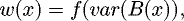
These new methods enabled to reconstruct indoor areas and eventually outdoor areas in real-time and 3D and also reconstruct 3D radioactive sources in volume. The sensor fusion method we developed can be considered as a proof of concept in order to evaluate the feasibility of performing nuclear measurement and radioactive sources localization algorithms in parallel. Furthermore, the benchmark that we will present as a conclusion of this communication enables to consider the reliability of radioactive source localization methods inputs.
In 2013, AREVA D&S started an R&D program for developing new investigation techniques based on autonomous sensing robotics and localization apparatus in order to provide new efficient exploration and characterization methods of contaminated premises and areas. This work corresponds to MANUELA® system developments by Areva D&S. Part of this work is protected by a patent (number WO2015024694) [3].
2 Materials and methods
2.1 General method
The presented method is based on two completely different techniques. The first one, which is called SLAM, is well known in the field of robotics, and it constitutes a specific branch of computer perception R&D. The second one, as described in [5,6], concerns radioactive sources localization and activity quantification from in-situ measurements and data acquisitions. The usual method for these acquisitions is time consuming for operators and, in consequence, integrated dose of workers during these investigations could be decreased.
Chen et al. [7] described such a mapping system based on merging RGBD-camera with radioactive sensors. The presented system automatically detects radioactive sources by estimating their intensities during acquisition with a deported computer using Newton's inverse square law (NISL). However, the NISL does not enable to estimate volumetric sources intensities; indeed, this calculation technique is limited to punctual radioactive sources relative intensity calculations.
Our aim was to build a complete autonomous system for being totally independent of any external features, and dependencies including GPS. Our set of constraints led us to implement the whole system in one single and autonomous apparatus. Our radioactive source localization processing is performed in two distinguished steps. First, we will research a probability of presence (geostatistics and accumulative signal back projection will help this interpretation) of radioactive source in order to estimate the source location and determine if it is volumetric or punctual. Second, after verification of the relevance of the acquisition, thanks to real-time uncertainties estimation, the operator will define source terms properties according to the acquisition (radionuclide signature and relative position of the sources and the device) and site documentation (radioactive source, chemical composition) in order to perform gamma transport inverse calculations. This way of computation principle leads to compute real volumetric radioactive sources activities and confidence intervals of the effective radioactive sources intensities.
A great problem for an autonomous apparatus (such as robot) is to locate itself in unknown environments, in order to compute appropriate motions and trajectories in volume. A simple formulation of this problem is that the apparatus must know its position in a map in order to estimate its trajectory. Using sensors, the system will build a map and compute its next position (translation and orientation in volume) at each acquisition step.
In order to compute SLAM inherent calculation in autonomous and light device development context, hardware specifications investigations are particularly important, due to required software performances.
2.2 Hardware
The presented radiological mapping system is embedded and designed for real-time investigations inside contaminated areas or premises. The whole system is enclosed and autonomous and needs no external marker or network for being active. However, the operator's real-time intervention requires real-time reconstruction and visualization, which is very performance-consuming.
2.2.1 Sensors
The system software input uses different sensors:
-
3D camera based on active stereoscopy. As shown in Figure 1, this camera's output consists of two different kinds of frame, a normal colour pixels image, and a depth map. The depth map is based on active stereoscopy technique and provides each colour pixel distance to sensor.
-
Nuclear measurements sensors including a dose rate meter and a micro CZT spectrometer (Fig. 2).
2.2.2 Computing unit
The 3D reconstruction and nuclear measurements are performed fully embedded, in real-time, due to operator interactions and acquisition time optimization in contaminated environment. Furthermore, the computing hardware must be fanless in order to avoid nuclear contamination. To satisfy these constraints, the embedded CPU must be enough powerful for supporting parallel processing.
 |
Fig. 1 Outcoming data from 3D sensor (left: depth-map, right: RGB image). |
 |
Fig. 2 Outcoming data from nuclear measurements sensors. |
2.3 Simultaneous Localization and Mapping
SLAM concept (Simultaneous Localization and Mapping) can be performed by merging different kinds of sensors; such as Inertial Measurement Units (IMU), accelerometers, sonars, lidars, and cameras. In our method, only 3D cameras are used. Using IMUs in order to improve our system accuracy is on of the main perspectives of our current developments. We propose to merge two different kinds of algorithms so as to reconstruct the environment in 3D, compute the trajectory with 6 degrees of freedom (translation, pitch, roll, and yaw) in volume, and merge measurements with the device's poses.
Two problems appear during that kind of acquisition. First, slight error during the odometry computation causes a non-regular drift of the trajectory. The second problem concerns the memory management of acquisitions in realtime. Indeed, 3D video gross data can quickly cost a considerable amount of active memory during the acquisition. Then, implementing a circular buffer is necessary for increasing the scanning volume up to hundreds of cube meters.
In order to develop our measurement method, we modified the RtabMap software [8–10] provided by IntroLab (Sherbrooke). By this way, we are able to use visual odometry with 3D cameras in order to reconstruct the environment and compute the device trajectory at 25 Hz.
Pose-graph visual SLAM is based on the principle that each acquisition step is a combination of constraints links between observations. These constraints are established using features detection and extractions of each processed image. This kind of SLAM problem is represented with graphs of constraints. Each observation of the robot creates node, new links and constraints. This method allows fast node recognition including loop and closure based on optimization methods.
2.3.1 Visual odometry
The goal of visual odometry is to detect the relative motion between two poses of the camera, and then to back-project the 3D and RGB streams in a computing reconstruction volume. This problem can be expressed as equation (1). This equation describes the transformation of each pixel of the camera to a 3D point, depending on intrinsic and extrinsic camera parameters:
 (1)
z: depth at pixel (u,v); u, v: coordinates of the considered pixel; fx: focal length along x; fy: focal length along y; cx, cy: lens centering on the optical axis; Ra,b: element of the rotation matrix; Ta: element of the translation vector; x, y, z: projected point coordinates in volume.
(1)
z: depth at pixel (u,v); u, v: coordinates of the considered pixel; fx: focal length along x; fy: focal length along y; cx, cy: lens centering on the optical axis; Ra,b: element of the rotation matrix; Ta: element of the translation vector; x, y, z: projected point coordinates in volume.
Visual odometry is processed on a real-time RGB-D data stream in order to detect the motions of the device in volume and get the colour for reconstruction. Simultaneously, the corresponding depth stream is used for calculating the rotation/translation matrix between two successive frames.
Visual odometry is features extraction based on. Each RGB image is processed in order to extract interest points. These interest points are formed by image corners. The corresponding pixel in the depth map is also extracted.
Depending on the pine-hole model, features are then back-projected in volume.
As described in Figure 3, unique correspondences are researched between two sets of consecutive images. If enough unique correspondences are detected, then odometry is processed. A RANdom SAmple Consensus (RANSAC) algorithm calculates the best spatial transformation between input images (rotation and translation).
 |
Fig. 3 Visual odometry processing. |
2.3.2 Loop and closure
Errors during the pose matrix computation cause a non-regular drift of the trajectory. Graph-SLAM and constrained optimization methods based on loop-and-closure correct this drift when a previously scanned zone is reached by adding constraints to previous acquired constraint graph as described in Figure 4 [8].
 |
Fig. 4 Loop and closure optimization. |
2.4 Nuclear measurement management and location
Measurements in motion-related work [11] by Panza describe a system used within motions in two dimensions with collimated measurements probes. In this case, using leads collimator could be possible, but our case concerns a handheld system measuring in a near 4pi sphere, and moving with six degrees or freedom.
All the data (nuclear measurement and positioning, 3D geographical and trajectory reconstruction) are performed in real-time while the device can have different kinds of status: moving or motionless. All the nuclear measurements are considered isotropic.
Each set of measurement (integrated or not) is attached to the Graph-SLAM geographical constraints structure. This allows performing trajectory optimizations and measurement positioning optimization simultaneously.
In order to satisfy the “real-time” constraint, a user interface displays every current measurement and process step in real-time in order to provide all pertinent and essential information to the operator (Fig. 5).
 |
Fig. 5 Acquisition interface. |
2.4.1 Continuous measurement
Dose rate measurements are processed during the 3D reconstruction with a lower frequency (around 2 Hz) than video processing (around 20–25 Hz). In order to manage the nuclear measurement positioning, we had to find a compromise between positioning uncertainty, which depends on the counting time and counting uncertainty that depends on the inverse counting time. So, first and foremost, dose rate measurement is positioned at half path distance during integration (Fig. 6).
Assigning radioactive measurements to a specific timeframe will cause a negligible error. The time measurement error in parallel processing is around a few milliseconds, and the minimal integration time for dose rate measurements is around 500 ms. The predominant measurement positioning uncertainty will be caused by the motion of the instrument during the integration of measurements and the linear poses interpolation method that is presented in Figure 6.
Gamma spectrometry measurements are processed with an even lower frequency (around 0.3 Hz) than the dose rate measurements (around 2 Hz). Consequently, the uncertainty on spectrum positioning is more important, compared to dose rate positioning. To compensate this error, dose rate values will help to distribute weighted spectrums for the acquired one (Fig. 7).
Considering the whole integration path, using high frequency IMU will help (in future developments) to locate measurements points more accurately during the capture by considering intermediate motions between the graph nodes.
 |
Fig. 6 Nuclear measurements positioning. |
 |
Fig. 7 Spectrum positioning management. |
2.4.2 Integrating measurement
In some case, very precise measurements are required to build a representative map of the environment. The fast pose calculation method we use allows considering the device as a 3D accelerometer with a higher frequency than nuclear measurements. While the 3D video stream is being acquired, the acceleration of the device is estimated and if the device is motionless, measurements can be integrated at the current pose (Fig. 8).
The main problem of this integration method is the lack of path looping consideration. Indeed, if the instrument trajectory crosses a previous location, this integration method is not sufficient to treat new measurements points at the previously considered integration zone. In order to manage new measurements and to improve measurements integration, efficient research of neighbour measurement points can be performed thanks to nearest neighbour research algorithms (e.g. kd-tree, etc.). Anyway, the gamma emitter decay half-life must be long enough to consider its radioactive activity unchanged during the measurement process. In order to correct this eventual decrease of nuclear activity, elapsed time between the beginning and the end of the measurement sampling process enables to estimate specific correction factors for each detected gamma emitter with the spectrometry measurements probe. This last principle could be explored as an important perspective of nuclear measurements real-time processing developments.
 |
Fig. 8 Radioactive measurements positioning. |
2.5 Near real-time post-processing, sources localization
At the end of acquisition, radioactive source localization computation methods are available with a set of algorithms that provide interpolations and back-projections of measured radioactive data in volume. The algorithms are optimized for providing results in a few seconds, even if uncertainties could be reduced by more accurate methods.
2.5.1 Measurements 3D interpolation
For interpolating measurements in 3D, we use a simple deterministic Inverse Distance Weighting (IDW) method, which is accurate enough considering the usual radioprotection operating accuracy. Furthermore, this fast computed method allows operators to consider the operating room state of contamination very quickly with this embedded method. The used IDW method is described within equations (2) and (3):
 (2)
with:
(2)
with:
 (3)v(x): interpolated value at x; wi: weight of the measurement point i;
  : distance between current interpolated point and measurement point i; n: number of measured points.
2.5.2 Dose rate back-projection
Back projection method is also deterministic and uses the 3D reconstruction to compute radiation emission zones in volume. This method is described within equations (4) and (5):
 (4)
(4)
 (5)
n: number of nuclear measurement point; B(x): back projection value (mGy h−1); x: location (x1,y1,z1) of back-projected value; X: location (x2,y2,z2) of nuclear measurement point; μa: linear attenuation coefficient of air (cm−2); w(x): weight associated to x location; DX,x: distance between X and x location.
(5)
n: number of nuclear measurement point; B(x): back projection value (mGy h−1); x: location (x1,y1,z1) of back-projected value; X: location (x2,y2,z2) of nuclear measurement point; μa: linear attenuation coefficient of air (cm−2); w(x): weight associated to x location; DX,x: distance between X and x location.
The back-projection algorithm inputs are:
-
3D reconstruction decimated point cloud;
-
nuclear measurements and position data.
Each point of the 3D point cloud (x in Eq. (4)) is considered as a possible radioactive source; then, emerging mean fluency or dose rate at the 3D reconstruction point (B(x) in Eq. (4)) is computed for every measured point (X in Eq. (4)). Further, variance distribution of the back-projected value enables to evaluate the possibility of radioactive source presence in volume at the back-projected point.
2.5.3 Topographical study
Topographical measurements can be performed as soon as the acquisition is terminated. This function gives instant information on the situation of premises.
2.6 Offline post-processing
The device output data can be processed in back office with a set of tools for estimating accurate gamma-emitting sources localization and quantification in volume. It also provides tools for estimating effects of a dismantling or decommissioning operation on dose rate distribution and allows the user to estimate the exposure of operators during interventions.
Next, subparagraphs will present these different tools such as radioactive sources quantification, operators' avatars, and topographic studies.
2.6.1 Topographical measurements
The dedicated post-processing software provides two kinds of topographical study tools, according to Figure 9: a global grid containing the scanned volume for global intervention prevision and a drag and drop tool for specific structure measurements (volumes, length, and thickness). These components enable to generate gamma transport particle simulations datasets in order to compute radioactive sources − measurements points transfer function, as described in Section 2.6.4.
 |
Fig. 9 Topographical study interface presenting dimensioning tools. |
2.6.2 3D nuclear measurements interpolation
Nuclear measurement interpolation characterization tool (Fig. 10) is based on IDW, and uses the same principle than the near real time post-processing interpolation method; however, slight modifications of scales allow user to refine the computation and then locate low emitting sources. Moreover, spectrometry can be exploited by interpolation user's defined region of interest of the spectrum. This enables specific studies concerning radionuclides diffusion in the investigated area, such as 137Cs or 60Co containers localization.
 |
Fig. 10 Radioactive measurements 3D interpolation. |
2.6.3 3D back-projection and avatar dose integration simulation
Back-projection algorithm also benefits of an improved interface in order to locate accurately radionuclides in volume using spectrometry (Fig. 11).
Avatars of operators can be used for estimating previsions of their exposure before operations. This dose rate integration estimation is performed by extrapolating dose rates from measurements points.
 |
Fig. 11 Radioactive measurements 3D back-projection. |
2.6.4 Sources activities estimations
Radioactive sources activities are estimated with a set of algorithms combining 3D transfer functions calculations and minimization methods (Fig. 12).
 |
Fig. 12 Radioactive sources activities estimation. |
2.6.4.1 Transfer function calculation
The transfer function will quantify the relation between volume radioactive source activities and resulting dose rate for a specific radionuclide.
The first step of radioactive sources estimation consists in modelling them according to available data provided by the results of acquisition on a hand, and by operating documents on the other hand (volume, enclosure type, shielding, materials, radionuclides) (Fig. 13).
In order to satisfy the nearest real-time calculation constraint, the transfer function calculation method is deterministic and based on ray-tracing and radioactive kernels point distribution in volume. Potential radioactive sources are designed by the user with the help of localization algorithm.
Equation (6) describes the transfer function calculation method.
 (6)
n: number of attenuating volumes on the ray path;
(6)
n: number of attenuating volumes on the ray path;  : dose rate at measurement point (considering the build-up factor); Av: volume activity of the radioactive source; C: dose rate − gamma fluency conversion coefficient; Bu: build-up factor for the “i” attenuating volume; μi: linear attenuation coefficient of the “i” attenuating volume; di: path length in the “i” attenuating volume; d2: total distance between the source kernel and the measurement point.
The numerical integration method for source kernels distribution in the source is a Gauss–Legendre integration based on method.
 |
Fig. 13 Radioactive sources scene modelling. |
2.6.4.2 Radioactive sources activities minimization method
The minimization method is based on iterative technique for which each step consists in considering a different combination of radioactive sources.
The equation system resolution method is based on the most important transfer function selection at each step of calculation.
Figure 14 presents the whole algorithm process for computing sources activities.
 |
Fig. 14 Minimization method algorithm. |
3 Benchmarks
Most of SLAM systems performances are compared thanks to Kitti dataset [12]. Nevertheless, Kitty dataset does not provide integrated comparison of nuclear sources localization systems merged to SLAM methods in real-time. In our case, we will need to estimate the reliability of our nuclear sources localization methods, which depend on the reliability of the trajectory and the topographical reconstructions with the 3D camera we integrated. To perform future comparisons between the sources localization methods we developed, the first step in this work consists in evaluating topographic and trajectory reconstruction reliability considering our constraints and parameters.
Since June 2016, a set of benchmarks is performed in order to compare the performances of this acquisition system with different systems that can be considered as references. Different parts of the system are compared such as:
-
3D volumetric reconstruction;
-
3D trajectory reconstruction;
-
dose rate measurements;
-
spectrometry measurements;
-
3D nuclear measurements interpolation;
-
3D radioactive source localization without collimator.
3.1 3D volumetric reconstructions
This part of the benchmark has been realized with a 3D scanner and is based on point cloud registration techniques such as Iterative Closest Points (ICP) method. We used “Cloud compare”, developed by Telecom ParisTech and EDF R&D department.
The reference point cloud was acquired with a 3D laser scanner from Faro Corporation (Tab. 1).
Comparison data.
3.1.1 Benchmark example
As an experimental test, we used a storage room “as it is” (Fig. 15).
 |
Fig. 15 Benchmark situation. Room dimensions: 25 m2, 2.5 m high. |
3.1.2 Results
Following clouds superposition pre-positioning, the ICP registration algorithm is performed in order to compute the best cloud-to-cloud matching. Then, point-to-point distance is computed for the whole reference point cloud.
Figures 16–18 show a part of the benchmark procedure.
The first step in Figure 16 concerns Faro® and MANUELA® point clouds superposition in order to prepare the matching process.
The second step consists in using ICP matching, and then computing point-to-point distances in the best matching case. In Figure 17, the colour scale displays the distribution of point-to-point distances between point clouds, and the chart shows the distribution of these distances in the whole scene.
The last graph displays the point-to-point distances distributions as a Gaussian (Fig. 18 shows the same chart as Fig. 17 with a different binning).
General conclusion of 3D point cloud reconstruction Benchmark shows a Gaussian distribution of cloud-to-cloud distance. Global cloud-to-cloud mean distance is around 7.3 × 10⁻² m (σ = 10.2 × 10⁻² m).
 |
Fig. 16 Faro (blue)/MANUELA® (RGB) point cloud superposition and registration. |
 |
Fig. 17 Cloud-to-cloud distance computation. |
 |
Fig. 18 Cloud distance diagram. |
3.2 3D trajectory reconstructions
The trajectory reconstruction is the support of nuclear measurements. In order to estimate these measurement localizations relevance in volume, we performed a few comparison of trajectories between our system based on RTABMap© SLAM library with our specific settings. The goal of this comparison is to prepare source localization algorithms reliability tests. Furthermore, this benchmark will be used in our future works in order to qualify the method of uncertainties estimation in real-time that we developed.
3.2.1 Materials and methods
The ground truth will be computed with a motion capture system. This motion capture system is based on Qualisys oqus 5+® devices. This provides a capture volume around 15 m3 (Fig. 19). In order to simulate higher acquisition volumes, the paths we captured were redundant with voluntary rejected loop detections. Furthermore, we will use the same methods than the one used in 3D reconstruction benchmark for estimating the difference between the reference method (computed with the motion capture system) and our instrument trajectory computation (ICP, distances distributions between trajectories point clouds).
 |
Fig. 19 Motion capture system simulation with visualization of the acquisition volume (blue) . |
3.2.2 Results
A few trajectory types have been acquired over 6 degrees of freedom in order to be representative of the real measurement acquisitions for nuclear investigations (straight line path, cyclic trajectories, and unpredicted paths, by different operators).
The most penalizing results are presented in Table 2.
These first results enable us to conclude that such kind of system is compatible with the geometric estimation performances which are needed during nuclear investigations of indoor unknown premises. These results will also enable us to compare our real-time uncertainties estimations method to experimental results and then validate the whole concept in the future.
Trajectory reconstruction comparison.
4 Uncertainties estimation
4.1 General considerations
Current work is ongoing for estimating uncertainties on each step of the acquisition.
Uncertainties estimation and propagation in such kind of acquisition and processing system are necessary for interpreting the results, estimating the relative probability of presence of radioactive sources, and building sensibility analysis in order to increase the system performance, by detecting the most uncertainty generator step in the process.
The whole process chain depends on four simple entries: the RGB image, the depth map, the dose rate measurements and the spectra measurements. Each one of these entry elements is tainted by systematic and stochastic uncertainties. Moreover, each step of process generates uncertainties and amplifies the input uncertainties.
In this paragraph, we will describe all parts of the acquisition process and present the basis of a new method we are developing for the uncertainties estimation of the whole process and measurements chain, in real-time. We compared this new method to a Monte-Carlo calculation that will be considered as the reference.
In the case of input detectors, we will only consider the model generated or counting (nuclear) measurement uncertainties.
4.1.1 Uncertainty estimation, general description
The acquisition and processing devices are decomposable in a few building blocks (sensor or processing technique). They will be considered separately in order to quantify each block uncertainty (Fig. 20).
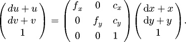
Each block will be considered as a linear system as described in equations (7) and (8):
 (7)
(7)
 (8)
O(u, v, w): output vector; T(ax,x, … , ax,x): transformation matrix; I(x, y, z): input vector.
(8)
O(u, v, w): output vector; T(ax,x, … , ax,x): transformation matrix; I(x, y, z): input vector.
Each of these blocks generates an intrinsic uncertainty and amplifies inputs errors. Then, the final ||dO|| will represent the global uncertainty on the acquisition and processing chain.
Each system uncertainty is considered as:
||dO|| = f (||dT||) error intrinsic generation estimation (Eq. (9))
 (9)
(9)
||dO|| = f (||dI||) error amplification estimation) (Eq. (10))
 (10)
(10)
We use Frobenius matrix norm (Eqs. (11) and (12)) in order to quantify the global variation of matrix terms.
 (11)
(11)
 (12)
(12)
 |
Fig. 20 Uncertainties propagation principle. |
4.1.2 Monte-Carlo methods
Monte-Carlo methods are efficient for propagating and estimating models uncertainties accurately. The main problem in such a method is computing time. This method will be considered as reference for comparison with the new method we developed. Furthermore, Monte-Carlo method will provide accurate results on each acquisition and process steps and will help to estimate how performances will be increased.
4.1.3 Interval arithmetic method
Interval arithmetic methods have been initially developed due to rounding errors of floating values in computing calculation. The principle is to describe a scalar value with an interval. This helps to consider irrational floating point values as duos of floating point scalar values with specific rounding policies. For example, π ∊ [3.14; 3.15].
This description of values will change arithmetic rules. For example, mathematical product becomes:

With this arithmetic, we developed a method for propagating uncertainties as boundaries of a noisy system. We will compare this method with Monte-Carlo uncertainties estimations method. We choose, as an example case, the 3D camera projection Matrix (pine-hole model).
4.2 3D Camera calibrations
The 3D camera output data is a duet of frames, a RGB one and a depth map. Each of them can be described as pinholes. Then, pixels 3D back-projections in volume are considered in equation (13):
 (13)
z: depth at pixel (u,v); u,v: coordinates of the considered pixel; fx: focal length along x; fy: focal length along y; cx, cy: lens centering on the optical axis; x, y, z: projected point coordinates in volume.
(13)
z: depth at pixel (u,v); u,v: coordinates of the considered pixel; fx: focal length along x; fy: focal length along y; cx, cy: lens centering on the optical axis; x, y, z: projected point coordinates in volume.
Values of interest in this models are (x,y,z) coordinates of the projected pixel. These coordinates, depending on features detection, will be processed in the VSLAM algorithm.
To provide interpretable results, the pinhole must be calibrated, and the calibration process will give interpretable back-projection uncertainties on (x,y) coordinates. Uncertainty on z coordinate will be estimated in the function of the depth, material and radioactivity level. Indeed, depth map is computed with active stereoscopy, which involves infrared coded grids projection and interpretations, which can be sensitive to external interferences.
4.2.1 Uncertainties estimations on camera calibration coefficients
The calibration of the camera consists in minimizing the pinhole projection matrix elements, using a well-known projection pattern.
The calculation of back-projections errors is performed with a Monte-Carlo random selection of calibration values cx, cy, fx, fy on one hand, and then, these back-projection errors are compared with intervals estimations. Deviations estimations methods are described with equations (14) and (15).
 (14)
(14)
 (15)
(15)
4.2.2 Monte-Carlo estimation
This method gives exhaustive results on the camera response, but it takes around 2 min to be computed for each frame, which is not suitable with real-time computations.
Figure 21 shows results of Monte-Carlo simulation varying the pinhole projection matrix elements; each matrix element could vary from −10 to +10%. 1E+6 random selections have been performed. The resulting error due to the lenses system will not cause a larger deviation than 80 pixels on the photographic sensor.
The second diagram (Fig. 22) shows the error amplification by the projection matrix. In this specific case, it does not have physical sense because it would represent the variation of a vertex coordinates as a function of pixel coordinate variation, which has no physical sense.
The pinhole model is linear; consequently, variation of output variation norms is distributed along a straight line.
The last diagram (Fig. 23) combines errors generated and amplified by the pinhole projection matrix. And this error will be considered as input error by the next processing block of the system (for each value of  ).
).
 |
Fig. 21 Monte-Carlo estimation of pinhole model uncertainties generation. |
 |
Fig. 22 Linear system error amplification by Monte-Carlo methods. |
 |
Fig. 23 Global uncertainties generated by the pinhole model. |
4.2.3 Intervals estimation
Provided results are less exhaustive than with Monte-Carlo methods; nevertheless, these results are bounding phase space provided by Monte-Carlo method. Furthermore, executing time is around 5 ms per frame, which is compliant with real-time analysis and processing.
Figures 24–26 show comparisons between uncertainties computed by Monte-Carlo and by intervals. This graphical representation represents the bounding of Monte-Carlo computed values by interval arithmetic method. Interval arithmetic results have been added to Monte-Carlo charts in order to figure both methods results (interval arithmetic results have been encircled to remain visible).
The simulation has been performed considering exactly the same matrix element variations. Indeed, matrix elements have been defined as intervals (Eq. (16)).
 (16)
(16)
Results in Figure 24 show a good concordance of both methods, and intervals arithmetic provides limits of Monte-Carlo method for intrinsic uncertainties generation.
Concerning the amplification of input system uncertainties, the input vector will be defined as a vector of intervals (Eq. (17)):
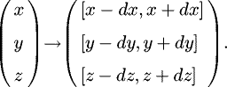 (17)
(17)
Depending on this definition of the input vector, intervals of the output vector will be estimated, as shown in Figure 25.
In this case, intervals also provide bounds of Monte-Carlo simulation.
Finally, by merging the system extrinsic and intrinsic parameters, a global estimation of generated uncertainties can also be provided with intervals techniques, by bounding Monte-Carlo values (Fig. 26).
 |
Fig. 24 Comparison between Monte-Carlo and intervals for estimating uncertainties of pinhole model. |
 |
Fig. 25 Comparison between Monte-Carlo and intervals for estimating uncertainties amplification by the pinhole model. |
 |
Fig. 26 Comparison between Monte-Carlo and intervals method for propagating the global uncertainties of the model. |
4.2.4 Performances benchmark
In this case, both methods can provide clear uncertainties results about input data uncertainties amplification and intrinsic uncertainties generation.
These methods can have different use of cases depending on each method's pros and cons.
The Monte-Carlo method will describe accurately the different systems, but interval arithmetic method can provide pertinent accuracy indices on each acquisition, in real-time or near real-time. Indeed, Monte-Carlo algorithm runs in around 2 min and interval arithmetic one runs in almost 5 ms in the same study case.
4.3 Radiological measurement
The second kind of algorithms input data are nuclear probes outcoming ones.
4.3.1 Dose rate measurements
Dose rate measurements uncertainties are linked to counting errors. Equations (18)–(20) describe the global dose rate counting error.
Count to dose rate pre-processing:
 (18)
with:
(18)
with:
 (19)and relative uncertainty is given by:
 (20)
(20) : dose rate; Cpm: count per minute; H: conversion factor mR h−1 to mGy h−1; Cps: count per second; τ: detector's dead time constant (s); Sd : detector sensibility coefficient (Cpm mR h−1); t: acquisition time (s); C: count during the acquisition time t in seconds; N: counting rate; u: relative uncertainty (%).
4.3.2 Spectrum measurements
Gamma spectrometry also depends on counting uncertainties. In this case, counting uncertainties are considered for each spectrometry channel. Spectrometry uncertainties also depend on energy/efficiency calibration quality and acquisition parameters.
4.4 SLAM method uncertainties
During SLAM acquisitions, each pose calculated by odometry and corrected by loop and closure algorithm is associated to a variance, due to statistical way of calculating spatial transforms which gives a confidence index on each pose computation. Concerning the 3D reconstruction, uncertainty will combine poses computations and 3D projection uncertainties.
4.5 Ongoing work
Current work concerns the estimation of each building-block uncertainties generation and amplification, such as depth map variations as a function of the environment conditions, spatial transforms variance due to descriptors variations, numerical applications of back-projection or geostatistical interpolation. Radioactive sources localization uncertainties generation and propagation will also be estimated in order to provide a complete method for estimating uncertainties and errors in such kind of system that combines acquisition of physical measurements and automatic processing in near real-time.
Also, a full benchmark of the system is performed in order to correlate its results with real-time uncertainties estimations. Each building block will be compared to well-known references systems. For example, in order to compare 3D reconstructions, we will use a Faro scanner as reference, and concerning trajectory computation, Vicon™ camera system will provide reference of spatial motions of the device.
5 Conclusion
The new-presented method for 3D Indoor/Real-time Topographical and Radiological Mapping (ITRM), with Visual Simultaneous Localization and Mapping (VSLAM) has been developed to perform near real time acquisitions and post-processing for radiological characterization of premises. Such method allows optimizations of operational time, personnel dose and waste minimization. One of the major challenges consists in optimizing the mobile experimental apparatus in order to satisfy the desired performances, by generating optimized programming code, selecting high performance computer units and measuring instrument. Such an optimization also needs a careful study of uncertainties introduced by the used instrumentation and developed algorithms. Indeed, physical measurement must be provided with associated uncertainty, in order to estimate its pertinence. Also, this uncertainties study method will finally enable performing a sensibility analysis of the whole system. Consequently, it will help to define the building blocks to improve and increase the system's performances.
More details about benchmarking and uncertainties estimations for such kind of data fusion systems will be presented in Hautot PhD thesis [13].
Finally, this new approach that we developed and applied for radiological measurements within the nuclear field could be of interest in other domains by adapting the sensors for the required measurements (chemical, environmental, etc.).
Acknowledgments
This ongoing work is funded by ANRT (Agence Nationale de la Recherche et des Technologies) under a CIFRE contract (number 2013/1542) between AREVA/STMI and CNRS.
References
- M. Morichi, H. Toubon, R. Venkataraman, J. Beaujoin, Ph. Dubart, Nuclear measurement technologies & solutions implemented during nuclear accident at Fukushima, in Proceedings of the IEEE/Advancements in Nuclear Instrumentation Measurement and their Applications (ANIMMA) International Conference (2013) [Google Scholar]
- T. Whelan, H. Johannsson, M. Kaess, J.-J. Leonard, J. McDonald, Robust real-time visual odometry for dense RGB-D mapping, in Proceedings of the IEEE International Conference on Robotics and Automation (ICRA) (2013), pp. 5724–5731 [Google Scholar]
- S. Izadi, D. Kim, O. Hilliges, D. Molyneaux, R. Newcombe, P. Kohli, J. Shotton, S. Hodges, D. Freeman, A. Davison, A. Fitzgibbon, KinectFusion: real-time 3D reconstruction and interaction using a moving depth camera, in Proceedings of the 24th Annual ACM Symposium on User Interface Software and Technology, ACM 2011, October (2011), pp. 559–568 [Google Scholar]
- J. Zhang, S. Singh, Visual-lidar odometry and mapping: low-drift, robust, and fast, in 2015 IEEE International Conference on Robotics and Automation (ICRA) (IEEE, 2015), pp. 2174–2181 [CrossRef] [Google Scholar]
- P. Dubart, M. Morichi, 3D topographic and radiological modeling of an environment, STMI International Patent Application WO2015024694, 2015 [Google Scholar]
- F. Hautot, Ph. Dubart, R. Abou-Khalil, M. Morichi, Novel real-time 3D radiological mapping solution for ALARA maximization, in IEEE/Advancements in Nuclear Instrumentation Measurement and their Applications (ANIMMA) International Conference, 2015, Lisbon (2015) [Google Scholar]
- L.-C. Chen, N.V. Thai, H.-F. Shyu, H.-I. Lin, In situ clouds-powered 3-D radiation detection and localization using novel color-depth-radiation (CDR) mapping, Adv. Robot. 28, 841 (2014) [CrossRef] [Google Scholar]
- M. Labbé, F. Michaud, Online global loop closure detection for large-scale multi-session graph-based SLAM, in Proceedings of the IEEE/RSJ International Conference on Intelligent Robots and Systems (2014) [Google Scholar]
- M. Labbé, F. Michaud, Appearance-based loop closure detection for online large-scale and long-term operation, IEEE Trans. Robot. 29, 734 (2013) [Google Scholar]
- M. Labbé, F. Michaud, Memory management for real-time appearance-based loop closure detection, in Proceedings of the IEEE/RSJ International Conference on Intelligent Robots and Systems (2011), pp. 1271–1276 [Google Scholar]
- F. Panza, Développement de la spectrométrie gamma in situ pour la cartographie de site, PhD thesis, Université de Strasbourg, 2012 [Google Scholar]
- A. Geiger, P. Lenz, C. Stiller, R. Urtasun, Vision meets robotics: the Kitti dataset, Int. J. Robot. Res. 32, 1231 (2013) [Google Scholar]
- F. Hautot, Cartographie topographique et radiologique 3D en temps-réel : Acquisition, traitement, fusion des données et gestion des incertitudes, PhD thesis, Université Paris-Saclay, 2017 [Google Scholar]
Cite this article as: Felix Hautot, Philippe Dubart, Charles-Olivier Bacri, Benjamin Chagneau, Roger Abou-Khalil, Visual Simultaneous Localization and Mapping (VSLAM) methods applied to indoor 3D topographical and radiological mapping in real-time, EPJ Nuclear Sci. Technol. 3, 15 (2017)
All Tables
All Figures
|
Fig. 1 Outcoming data from 3D sensor (left: depth-map, right: RGB image). |
| In the text | |
|
Fig. 2 Outcoming data from nuclear measurements sensors. |
| In the text | |
|
Fig. 3 Visual odometry processing. |
| In the text | |
|
Fig. 4 Loop and closure optimization. |
| In the text | |
|
Fig. 5 Acquisition interface. |
| In the text | |
|
Fig. 6 Nuclear measurements positioning. |
| In the text | |
|
Fig. 7 Spectrum positioning management. |
| In the text | |
|
Fig. 8 Radioactive measurements positioning. |
| In the text | |
|
Fig. 9 Topographical study interface presenting dimensioning tools. |
| In the text | |
|
Fig. 10 Radioactive measurements 3D interpolation. |
| In the text | |
|
Fig. 11 Radioactive measurements 3D back-projection. |
| In the text | |
|
Fig. 12 Radioactive sources activities estimation. |
| In the text | |
|
Fig. 13 Radioactive sources scene modelling. |
| In the text | |
|
Fig. 14 Minimization method algorithm. |
| In the text | |
|
Fig. 15 Benchmark situation. Room dimensions: 25 m2, 2.5 m high. |
| In the text | |
|
Fig. 16 Faro (blue)/MANUELA® (RGB) point cloud superposition and registration. |
| In the text | |
|
Fig. 17 Cloud-to-cloud distance computation. |
| In the text | |
|
Fig. 18 Cloud distance diagram. |
| In the text | |
|
Fig. 19 Motion capture system simulation with visualization of the acquisition volume (blue) . |
| In the text | |
|
Fig. 20 Uncertainties propagation principle. |
| In the text | |
|
Fig. 21 Monte-Carlo estimation of pinhole model uncertainties generation. |
| In the text | |
|
Fig. 22 Linear system error amplification by Monte-Carlo methods. |
| In the text | |
|
Fig. 23 Global uncertainties generated by the pinhole model. |
| In the text | |
|
Fig. 24 Comparison between Monte-Carlo and intervals for estimating uncertainties of pinhole model. |
| In the text | |
|
Fig. 25 Comparison between Monte-Carlo and intervals for estimating uncertainties amplification by the pinhole model. |
| In the text | |
|
Fig. 26 Comparison between Monte-Carlo and intervals method for propagating the global uncertainties of the model. |
| In the text | |
Current usage metrics show cumulative count of Article Views (full-text article views including HTML views, PDF and ePub downloads, according to the available data) and Abstracts Views on Vision4Press platform.
Data correspond to usage on the plateform after 2015. The current usage metrics is available 48-96 hours after online publication and is updated daily on week days.
Initial download of the metrics may take a while.