| Issue |
EPJ Nuclear Sci. Technol.
Volume 4, 2018
|
|
|---|---|---|
| Article Number | 13 | |
| Number of page(s) | 17 | |
| DOI | https://doi.org/10.1051/epjn/2018009 | |
| Published online | 22 June 2018 | |
https://doi.org/10.1051/epjn/2018009
Regular Article
A methodology for performing sensitivity analysis in dynamic fuel cycle simulation studies applied to a PWR fleet simulated with the CLASS tool
1
Subatech, IMTA-IN2P3/CNRS-Université,
44307
Nantes, France
2
IRSN/PSN-EXP/SNC/LNC,
BP 17,
92262
Fontenay-aux-Roses, France
3
Institut de Physique Nucléaire d’Orsay, CNRS-IN2P3/Univ. Paris-Sud,
Orsay, France
4
CEA, DEN, Cadarache, DER, SPRC/LECY,
13108
Saint-Paul-lez-Durance, France
5
Univ. of Wisconsin Madison, Department of Nuclear Engineering and Engineering Physics,
Madison,
WI, USA
6
Laboratoire de Physique Subatomique et de Cosmologie, Université Grenoble-Alpes, CNRS/IN2P3,
Grenoble, France
* e-mail: This email address is being protected from spambots. You need JavaScript enabled to view it.
Received:
23
August
2017
Received in final form:
15
January
2018
Accepted:
3
April
2018
Published online: 22 June 2018
Abstract
Fuel cycle simulators are used worldwide to provide scientific assessment to fuel cycle future strategies. Those tools help understanding the fuel cycle physics and determining the most impacting drivers at the cycle scale. A standard scenario calculation is usually based on a set of operational assumptions, such as reactor Burn-Up, deployment history, cooling time, etc. Scenario output is then the evolution of isotopes mass in the facilities that composes the nuclear fleet. The increase of computing capacities and the use of neutron data fast predictors provide new opportunities in nuclear scenario studies. Indeed, a very high number of calculations is possible, which allows testing a high number of operational assumptions combinations. The global sensitivity analysis (GSA) formalism is specifically well adapted for this kind of problem. In this new framework, a scenario study is based on the sampling of operational data, which become input variables. A first result of a scenario study is the highlight of relations between operational input data and outputs. Input variable subspace that satisfy optimization criteria on an output, such as plutonium incineration or stabilization, can also be determined. In this paper, a focus is made on the methodology based on GSA. This innovative methodology is presented and applied to a simple fleet simulation composed of a PWR-UOx fuel and a PWR-MOx fuel. Calculations are done with the fuel cycle simulator CLASS developed by the CNRS/IN2P3 in collaboration with IRSN. The design of experiment is built from five fuel cycle input sampled variables. Sensitivity indices have been calculated on plutonium and minor actinide (MA) production. It shows that the PWR-UOx Burn-Up and the fraction of PWR-MOx fuel are the most important input variables that explain the plutonium production. For the MA production, main drivers depend strongly on isotopes. Sensitivity analysis also reveals input variable subspace responsible of simulation crash, what led to an important improvement of the model algorithms. An equilibrium condition on the plutonium mass in the stockpile used for building MOx fuel has been applied. The solution is represented as a subspace in the PWR-UOx Burn-Up and PWR-MOx fraction input space. For instance, achieving a plutonium equilibrium in a stockpile fed by a PWR-UOx that operates at 40 GWd/t requires a PWR-MOx fraction between 9 and 14%. This study also provides data related to plutonium incineration induced by the utilization of the MOx.
© N. Thiollière et al., published by EDP Sciences, 2018
 This is an Open Access article distributed under the terms of the Creative Commons Attribution License (http://creativecommons.org/licenses/by/4.0), which permits unrestricted use, distribution, and reproduction in any medium, provided the original work is properly cited.
1 Introduction and motivations
Fuel cycle simulators associated to innovative analysis methodologies are developed for enhancing the scientific knowledge on nuclear fuel cycle physics. By calculating radioactive inventory evolution in each unit of an evolving fuel cycle, dynamic fuel cycle tools help understanding fuel cycle physics highlighting the drivers for each specific output observable. Also, an electro-nuclear fuel cycle scenario study is connected to other energy and electricity production sources. Many scientific fields may be involved, such as economy, sociology, etc. Fuel cycle simulators are then useful tools for building interdisciplinary researches in link with scientific fields mentioned above. As a consequence, technical and interdisciplinary researches on fuel cycle produce analysis that could help enlighten the debate and the decision making process in the context of the energy transition.
A lot of different fuel cycle simulation tools are developed by nuclear engineering and research institutions. Several level of detail are reached by available tools, from the simple spreadsheet to a complex code. This complexity depends on the reactor type or fuel characteristics. For innovative reactors, such as GEN IV reactors, as for reprocessed fuel such as advanced MOx fuel, a high level of reactor physics is required to ensure a high level of confidence in results. Nuclear energy policy is usually part of a national strategy. This is why a lot of scenario studies based on nuclear fuel cycle simulators are focused on the country scale, taking into account the country specificities [1–3]. Nevertheless, some dedicated studies could be also extended to continent in the case of high relationship level between countries, as Europe for instance [4].
In France, the most advanced software for fuel cycle simulations is the code COSI [5], developed by CEA1. The physics is represented with a very high level of detail. At the international level, a lot of tools are available. For instance, the agent-based nuclear fuel cycle simulation Cyclus [6] is developed and used for a large range of applications: non-proliferation [7], nuclear archeology [8], etc. The code VISION [9] developed by DOE laboratories is used in the framework of the system analysis working group of the United States research program on advanced fuel cycles. We can also mention the code EVOLCODE [10] developed by the CIEMAT2, the code DANESS (Dynamic Analysis of Nuclear Energy System Strategies) [11] developed by the international operating expert firm Nuclear21, and many others.
A lot of work has already been produced on input variables uncertainty propagation. The nuclear data uncertainty propagation in nuclear fuel cycle simulation outputs has been assessed [12]. The Nuclear Energy Agency Expert Group on Advanced Fuel Cycle Scenarios has produced a study to evaluate the effects of the uncertainties of input parameters on the outputs of fuel cycle calculations [13].
The present paper represents a continuation of the effort described below. The main innovation is the definition of a complete design of experiment that leads to a relative high number of fuel cycle simulations. In this representation, input parameters are not considered as uncertainties, but as scenario study results that fit with selection criteria imposed on outputs.
Usually, nuclear fuel cycle scenario studies are based on few very detailed simulations. Reactors and other fuel facilities parameters are defined by the user. Reactors could be defined by the thermal power, the specific power and the discharge Burn-Up. The physics related to the reactor depends on the characteristics of the core such as geometry, composition and temperature. Mean cross sections needed for solving the evolution equations are processed from the neutron spectrum. A new technology deployment plan is defined by the deployment date and the deployment kinetic, usually optimized from several upstream calculations. Input variables are called scenario assumptions and their choice strongly impacts the output analyses and then, the scenario evaluation.
The last generation of fuel cycle simulation tools has been developed in order to be fast. The codes processing speed as well as the increase of the computing capacities open a new paradigm for fuel cycle simulator utilization, since a very high number of calculations could be achievable.
The present work shows how to build and assess a simple nuclear scenario, from tools provided by the sensitivity analysis. The method supposes to build a design of experiment in which input variables are sampled. Sensibility indices are used to select the most impactive variables on an specific output which helps to guide the analysis. The effect of input variables on model outputs could be determined and quantified. Finally, this methodology provides also solution spaces from any criteria on output observable. The paper presents also an illustration of the method with an adapted design of experiment used to study a simplified PWR-UOx MOx fuel fleet. The focus is made here on the methodology precise description, and on some relevant results.
The GSA is described and its contribution on fuel cycle studies is highlighted. Then, the fuel cycle simulator CLASS, used as the fuel cycle model for the sensitivity analysis study performed on a simplified PWR UOx and PWR MOx fleet is presented. This methodology can be used on any fuel cycle strategy evaluation. The design of experiment is described, as the methodology for storing and analyzing output data. Finally, input variables impact on plutonium and minor actinides (MA) production will be presented.
2 Global sensitivity analysis for fuel cycle studies
This section aims to describe the framework of the fuel cycle simulations used to build the analysis study of a simplified PWR-UOx MOx fleet. The current methodology used for building scenario studies is explained and the global sensitivity analysis (GSA) innovative contribution is detailed.
2.1 Dynamic fuel cycle studies
A fuel cycle simulation is usually based on a complex computer code that models material irradiation in reactors, cooling phases and exchanges in facilities. Most important effort concerns, in the neutron physics point of view, the fresh fuel composition needed to reach reactor requirements and the calculation of the composition according to the irradiation conditions.
The fresh fuel determination is usually based on a fuel loading model (FLM) that aims to provide fractions of materials needed to satisfy reactor requirements (maximal Burn-Up, regeneration rate, etc.) for any available materials. This could be achieved for instance by a simple formula, by the use of 239Pu equivalent methods [14] or with neural network based predictors [15]. An additional algorithm is then needed to determine the appropriate composition built from available stocks.
Once the fresh fuel is built, the model calculates the evolution of materials under neutron irradiation. The calculation scheme is based on the resolution of the two following equations:
-
the Boltzmann equation provides the neutron spectrum which leads to the mean cross sections calculation;
-
the Bateman equations are the isotopic vector evolution equations solved from initial composition and specific thermal power.
In practice, the coupling between those two equations leads to precise calculated inventory. Indeed, when the composition is evolving, neutron spectrum has to be frequently updated in order to use correct mean cross sections. To precisely simulate fuel evolution in a fuel cycle simulator, two methods are usually used. The first one consists to build a coupling with a neutron transport code which includes also a Bateman equations solver. This solution is very accurate but requires a high computing time. The second solution consists in building and using neutron data predictors in the fuel cycle simulation. The advantages of predictors is that computing time is very fast compared to neutron code coupling. Nevertheless, a minimum bias in comparison with the reference calculation must be guaranteed.
A fuel cycle simulator integrates several spatial and temporal scales connected to different physics phenomena:
-
nuclear reactions induced by neutrons flux;
-
nuclear core isotopic composition evolution under the neutron flux;
-
nuclear fleet transition induced by reactor deployment or phase out;
-
middle and long term inventory activity decay.
As a consequence, a dynamic fuel cycle simulation output may be characterized by a high uncertainty, with several origins that could be classified as follow:
-
nuclear data used to calculate neutron flux and mean cross sections;
-
reactors (resp. cycle) simplifications in the transport (resp. fuel cycle) simulations;
-
operational assumptions imposed in the fuel cycle simulation.
The nuclear data include microscopic cross sections, fission and decay data used in the transport code. Effect of nuclear data uncertainties on a fuel cycle output has been investigated in [12]. Reactor simulation simplifications are coming from the difficulties to simulate precisely a full core reactors taking into account all the specificities (irradiation history, reactivity control with boron or control rods, fuel loading patterns, etc.). The common methodology for fuel cycle simulations consists in using assemblies with mirror conditions, which leads to increase uncertainty. The impact of using assembly calculation has been investigated in [16]. Fuel cycle simplifications could be part of the model or decided by the user during the scenario construction. Among them, we can point for instance first loadings after reactor operation starting date, shutdown of unit duration during fresh fuel loadings, etc. The impact of those kind of simplifications should be quantified in the future.
Operational assumptions are operational data that are user-defined in a fuel cycle simulation. That could be reactor Burn-Up, thermal power, loading factor, deployment date or other facility characteristics. Those kind of data could not be determined since fuel cycle simulators aims to model future trajectories. The utilization of neutron data predictors and the increase of computing capacities provide new opportunities to perform nuclear scenario studies since a very high number of calculations is currently reachable. In this new vision, operational assumptions are not unknown data but become scenario results obtained by applying optimization criteria on scenario outputs. In a longer-term perspective, this methodology based on a multi-criteria analysis that would take into account technical, economical and even sociological criteria could be considered.
Massive fuel cycle simulation requires a suitable mathematical framework and GSA fulfills perfectly this role.
2.2 Global sensitivity analysis (GSA)
GSA is used in many research fields involving modeling of complex physical phenomena. Each field applies GSA according to its specific needs. A lot of relevant bibliographical sources are available, for instance [17–19]. According to [20], GSA provides relevant answers for following applications:
-
test if the model is in agreement with the simulated process;
-
determine most impacting input variables on an output observable variability;
-
highlight negligible input variables or model parameters;
-
highlight and understand interactions between variables.
For fuel cycle simulators applications, GSA could also help understanding the physics from input and output variables relations highlight. In addition, it could provide relevant informations for detecting and correcting errors in the code algorithms.
For application involving a lot of variables with potential interactions, variance based methods are powerful and suitable tools. A lot of sensitivity indices may be used. Since fuel cycle studies have a high input data number and spread, output observables (such as plutonium mass at a given time) may have a high variability. Sobol’ indices are efficient estimators of input variables or model parameters weight in an output variability and have been chosen in the framework of the proposed application (see Sect. 4.2).
2.3 Design of experiment
The fuel cycle simulation used to illustrate the methodology describes a simplified nuclear fleet composed by PWR loaded with uranium oxide (UOx) and mixed oxide (MOx) fuels. Since the goal of the work is to study impact of reactor parameters on fuel cycle simulation outputs, one reactor of each type (UOx and MOx) is defined. It has been shown [1] that this kind of simplifications produced results that could be extrapolated to complex fleet simulation with reasonable accuracy. The MOx fuel integration impact will also be assessed by sampling the PWR-MOx fraction. Total thermal power at beginning of scenario is 2.1 GWth (2.8 GWth with a load factor of 0.75) and total heavy nuclei mass is 72.3 tons. During the calculation, reactors power and mass can be modified but the specific thermal power remains constant. Simulations schematic representation is shown in Figure 1.
An infinite stock feeds with natural uranium a fabrication plant that provides enriched uranium to the PWR-UOx reactor. Uranium enrichment is calculated from reactor required Burn-Up. An irradiation cycle is done and the spent UOx fuel is sent to the pool. After a cooling time defined by the user, the spent fuel is sent to a stock that is used by the MOx fabrication plant to build PWR-MOx fresh fuel. The fabrication plant separates the plutonium needed and add depleted uranium. During the separation process, the reprocessing losses are 0. The plutonium fraction in the MOx fuel is calculated to satisfy the required Burn-Up. The MOx fuel is irradiated in the reactor and sent to a pool and a stock after the cooling time. The power of the fleet is supposed to be constant during the scenario that end after 100 years of operation. Nevertheless, this condition can not always be realized because of the availability of the plutonium, as discussed in Section 4.3. In practice to simplify calculations, reactors lifetime has been set at the duration of the scenario. If this is not realistic from the technical point of view and if we could have defined more reactors, this has no impact on the inventory evolution calculation. Between t = 0 and t = 20 years, one PWR-UOx is operated and the plutonium builds-up in the stockpile. At t = 20 years until the end of the scenario at t = 100 years, a fraction of the total power is distributed to a PWR-MOx reactor.
Simulations were done with the fuel cycle simulator CLASS, described in Section 3. A set of five input variables of the fuel cycle simulation has been selected. Each input data has been uniformly sampled between a minimum and a maximum value that seems reasonable according to technological knowledge. Table 1 presents sampled input data with minimum and maximum value.
The Burn-Up of reactors are sampled independently between 30 and 60 GWd/t. The PWR-MOx fraction represents the PWR-MOx thermal power divided by the total thermal power and has been sampled between 0 and 20%. The PWR-UOx spent fuel is sent to the Pool-UOx and leaves after a cooling phase sampled between 0 and 20 years. During this time, spent fuel can’t be used to create new fuel. After the cooling time, each spent fuel is sent to stockpile and is available for fresh fuel fabrication. Two fuels management strategies have been tested. The FiFo (First in First out) strategy uses in priority the older fuels for building fresh fuel while the LiFo (Last in First out) strategy uses latest ones.
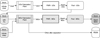 |
Fig. 1 Schematic representation of fuel cycle simulations. |
Input data range.
2.4 Simulations methodology and output data storage
The number of fuel cycle runs could be limited from:
-
the computing time;
-
the random access memory (RAM) utilization;
-
the data storage.
For such a calculation (two reactors during 100 years), the CLASS tool is very fast and around two minutes per CPU are required to run a single calculation based on precise neutron data predictors with a very small RAM request. The parallel batch computing farm we have used could run 200 simultaneous calculations. As a consequence, around 150 000 calculations per day could be run, which shows that computing time is not a limitation for this kind of Design of Experiment. For showing how data storage is the main limitation, we present methodology used to store informations.
After N CLASS simulations, a single file containing all the run informations is built. The output file is handled by the analysis software ROOT [21]. A ROOT TTree is built according to the structure represented in Figure 2.
Scalar data are connected to oval shape since data connected to square boxes are vectors in which index represents the time step. For reactors output data, in addition to inventory, the number of fresh fuel loading and missed loadings is stored. In the defined design of experiment, there is an empty cycle if there is not enough plutonium to operate the PWR-MOx. The number of missed loadings is then important for identifying runs with lack of plutonium in the stockpile.
According to the accepted memory size dedicated to the data file, around 10 000 simulations may be run. The set of output files generated by CLASS simulations is around 300 GB and the final output file size is close to 15 GB. A limitation coming from data storage memory may appear. Indeed, a full analysis study may require many simulation sets. To give an example, one could calculate the influence of a model parameter on results provided by an output file. This means to calculate and to store several high size files or directories, just for one simple nuclear fleet. Among solutions for the future of this methodology, we could investigate on selecting data to store, define the appropriate number of runs according to input variables and output variability, etc.
Two independent input variable samples have been generated from latin hypercube sampling (LHS) [22]. For calculating Sobol’ indices (see Sect. 4.2), a specific design of experiment composed by 15 000 runs obtained from two independent LHS samples of 1500 sets of input data has been used. For output direct analysis (see Sects. 5 and 6) as for preliminary analysis (see Sects. 4.3 and 4.4), 10 000 input data set have been sampled on a LHS.
 |
Fig. 2 Input and output data tree structure. |
3 The fuel cycle simulator CLASS
The fuel cycle model used in this work is the CLASS code [23] which is a dynamic fuel cycle simulation tool developed by CNRS3/IN2P34 in collaboration with IRSN5. The aim of CLASS is to model an evolving electro-nuclear fleet. The main output is the evolution of isotopes everywhere in the fleet. An economic module [24] is also currently developed to calculate the levelized cost of electricity of a nuclear fleet, from the start until the dismantling.
3.1 CLASS principle
The CLASS model is a collection of C++ classes that describes facilities in a nuclear fleet. The CLASS model has been built around the reactor class that drives radioactive material flows from reactor front to back end. Figure 3 lists current existing facilities and links between them.
Five facilities, listed in Table 2 with associated user defined parameters, are currently taken into account in CLASS. From its starting time and at each new loading, reactor requests a fresh fuel to the fabrication plant. The fuel is irradiated in the reactor and sent to the pool until the end of the cooling time. The pool could be connected to a separation plant, that send separated elements to stocks. The end of the path for any materials is a stock, that could be waste or not.
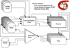 |
Fig. 3 Schematic principle of the CLASS library. |
Facility parameters in the CLASS code.
3.2 Reactor models
Reactor simulation in CLASS is defined by three models:
-
the FLM aims to build a fuel according to reactor requirements and stocks isotopic composition;
-
the cross section predictor (CSP) provides mean cross sections needed to solve the evolution equations during irradiation in the reactor;
-
the Bateman solver is a set of methods used during reactor irradiation for solving Bateman equations.
The FLM and the CSP are based on neutron data fast predictions, such as keff or mean cross section at a given irradiation time. For building predictors, a reactor data bank composed by several thousands of reactor evolution simulations is built and artificial neural networks are trained on neutron data outputs from initial fuel compositions at beginning of cycle (B.O.C.). Multi-Layer Perceptron from the library TMVA [25] is used with success for this purpose. It has been shown [15] that neural network neutron data prediction precision is close to Monte-Carlo uncertainty in the standard range of application.
At this time, several reactor models have been implemented in CLASS. An important part of the effort has been focused on PWR reactors loaded either with UOx or MOx fuel. More recently, a PWR loaded with MOx fuel on Enriched Uranium Support (MOXEUS) model is being developed for the study of plutonium multi-reprocessing in PWR. A PWR model based on MOx mixed with americium fuel has been also developed recently [26]. A sodium fast reactor (SFR) model has been built but further developments are needed and an important effort is currently made. In the future, other reactor models will be implemented, such as Small Modular Reactor, ADS or CANDU models.
3.3 CLASS improvement from GSA
Among all the runs obtained from the LHS sample, some crash and produce corrupted output files that cannot be read. From input variable space identified to produce corrupted files, a model improvement has been performed in the FLM related to the MOx fuel. Figure 4 shows crashed runs according to PWR-UOx Burn-Up and PWR-MOx fraction which are the most representative input variables for crashed runs identification. 852 simulations have crashed and the representation shows it appears mainly when the PWR MOx thermal power fraction and Burn-Up are high. Based on this observation, the development of a new FLM has solved the issue. All the simulations run properly with the design of experiment re-processed in the same conditions.
The new fuel algorithm is the main recent modification in the CLASS code. The CLASS version 5, in which the FLM will be described in detail, will be released soon. This application was presented in order to show how a sensitivity analysis based on an appropriate design of experiment can provide relevant informations for improving the fuel cycle simulator. All following analyses are based on calculations performed with the FLM of CLASS version 5.
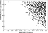 |
Fig. 4 Corrupted events according to PWR-UOx Burn-Up and PWR-MOx thermal power fraction in the total thermal power. This plot has been obtained with the previous CLASS version before the improvement of the FLM. |
4 Sensitivity indices estimation
The basic sensitivity evaluation usually focuses at estimating the alone effect of one input variable (while fixing all others) on the output. This approach gives information on the local effect of each variable, marginally. But when the range of input variables increases significantly, no reference or "center" point remains pertinent, and thus we aim at a global sensitivity effect of each input variable, and if possible of their combinations. Therefore, traditional indices like  are to be replaced by an averaged effect of Xi over {[X1min, X1max], [X2min, X2max], … , Xi, … , [Xpmin, Xpmax] }.
Sobol’ indices are a standard answer to this issue, standing on providing a probabilistic density/weighting of each Xi on its support interval [Ximin, Ximax]. This section aims to present Sobol’ indices formal definition and estimation. This is followed by a preliminary analysis on the LHS sample in order to avoid bias in the interpretation of simulations.
4.1 Sobol’ sensitivity indices
In the case of independent random input variables, it is possible to calculate sensitivity indices that represents each input variable contribution to the variability (variance) of the output. Such Sobol’ indices [19] are even more relevant because they also provide an access to interactive input variable contribution. We consider input variable Xi with i from 1 to p, with p the number of input independent variables. Index ij is related to the interaction between variables i and j. Index ijk represents three variables i, j, and k interaction, and so on.
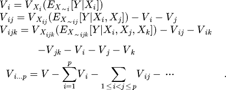
Sobol’ indices expression is based on the variance decomposition theorem [20]:
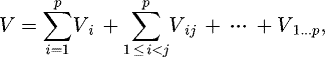 (1)
where V is the variance of the output Y. In the following, we call
(1)
where V is the variance of the output Y. In the following, we call  the variance of the conditional expectation of the output Y. Terms of the decomposition are given by:
 (2)
(2)
In those mathematical expressions, the notation Xi means varying Xi alone, since X∼i indicates that the set of all variables is varying except Xi. From this decomposition, Sobol’ indices of increasing order can be defined. The first order Sobol’ indices is given by:
 (3)
(3)
The second order Sobol’ indices represents variability of Y induced by interaction between input variable i and j:
 (4)
(4)
Higher order indices are built from the same scheme. All those indices are positive and according to equation (1), they are lower than 1. The higher the index is, the higher the input variable impact in the output variability is. The number of indices Nind to calculate is then linked to the number of input variable p with the following relation: Nind = 2p − 1. This relation leads to a very important number of order to calculate if the number of variable is high. According to Table 1, 4 numeric input variables leads to 15 Sobol’ indices by output variable for one fuel strategy. Since many output variables are important, this leads to a high number of Sobol’ indices to consider. Finally, Sobol’ total indices for each input variable can be calculated as follow:
 (5)
(5)
Sobol’ total indices measures the contribution of the variable i, alone and with all possible interactions with the others, in the variability of the output Y.
4.2 Sobol’ sensitivity indices estimation
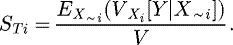
Sobol’ indices have been estimated for the plutonium production and the MA total production at the end of scenario, at t = 100 years. For this purpose, the specific design described in Section 2.4 has been used. It has been generated from the function sobolSalt [27] from the package sensitivity [28] of the analysis framework R [29]. This specific design has been used to calculate Sobol’ first-order, second-order and total indices. Sobol’ first order and total indices calculated by this method are presented in Table 3. Associated standard error provided by the model is 5% at maximum, which fixes the order of magnitude for indices validation limit.
Sobol’ indices estimation clearly shows that two input variables (PWR-UOx Burn-Up and PWR-MOx fraction) are the most impactive input variables. PWR-MOx fraction is the main driver for plutonium production at the end of scenario. The sum of first order Sobol’ indices for PWR-MOx fraction and PWR-UOx Burn-Up is 0.97 which means almost all the variability of the plutonium mass at the end of scenario is explained by those two variables. MA Sobol’ indices show that the spent UOx fuel cooling time also plays a non-negligible role, especially for LiFo strategy. Americium is the MA that induces this behavior. This will be investigated in Section 6.2. Neptunium production’s main driver is the PWR-UOx Burn-Up. Curium production is mainly explained by the PWR-MOx fraction and the PWR-UOx Burn-Up, but also by the PWR-MOx Burn-Up. Table 3 provides input variable prioritization that will be used for further detailed analyses.
The difference between 1st order and total indices is usually weak, especially for plutonium, neptunium and curium. This indicates that input variable interaction in the output is small [17]. Nevertheless, non-negligible difference appears for MA that can be explained by the americium. For assessing interaction between input variables, second order indices have been estimated from the same function. Uncertainty of the Monte-Carlo method is lower than 3%. In order to highlight important interaction effects, only second order higher than 0.05 are mentioned in Table 4.
Highest value of second order indices always involves input variable number 3, which is the PWR-MOx fraction, which means this variable has strong interactions with others. This can be interpreted by the fact that a small PWR-MOx thermal power decreases (resp. increases) PWR-MOx (resp. PWR-UOx) effects.
Sobol’ first order and total indices estimation. Four input variables are in column. Fuel strategy is specified if there is more than 5% difference between indices. The mention "All" means there is no difference between fuel strategies. Only indices higher than 0.05 are represented. PWR Burn-Up are mentioned (UOx BU and MOx BU), as the PWR-MOx thermal power fraction (Fr. MOx). CT UOx is the spent UOx cooling time.
4.3 PWR-MOx missed loading
This section is related to the analysis of PWR-MOx missed loading. PWR-MOx fuel missed loadings are due to a lack of available plutonium in the dedicated stockpile. Indeed, the FLM could not find enough Pu in the stockpile to build a fuel that reach the targeted Burn-Up, so no fuel at all is loaded and there is an empty reactor cycle. A missed load is not directly detected in the PWR-MOx fraction input variable and could induces a bias in the interpretation of results. As a consequence, only simulations without missed loading will be used as valid simulations for further inventory analysis. To analyze the role of input variables specified in Table 1 on the number of missed loading, this output is plotted according to main contributors in Figure 5.
The PWR-MOx missed loadings distribution (up and left plot), represented with a log scale, shows a majority of runs has no missed loadings at the end of scenario (t = 100 years). 3924 simulations among 10 000 have no missed loading. Other PWR-MOx missed loadings are distributed between 1 and 19. Other plots show the impact of other variables.
The number of runs with zero missed loadings decreases with the PWR-UOx Burn-Up (up and right plot). This is an effect of the first PWR-MOx loading. If the PWR-UOx Burn-Up is high, the cycle time is high since the reactor specific power is constant. For a higher cycle time, the probability to have a missed first loading for the PWR-MOx which starts at t = 20 years is higher. For high value of missed loadings (higher than 5), the distribution dependency with PWR-UOx Burn-Up is reversed. The higher the Burn-Up is, the higher the number of missed loadings is. This is a plutonium production rate effect. For a higher PWR-UOx Burn-Up, the plutonium production rate is lower since the production slope decreases with the Burn-Up. As a consequence, the averaged plutonium production per year is lower. A high PWR-UOx Burn-Up means a smaller plutonium amount in stockpile used by the PWR-MOx fabrication plant, which induces a higher missed loadings probability.
The number of runs with zero missed loadings does not clearly depends on the PWR-MOx Burn-Up (bottom and left plot). For number of missed loadings between 1 and 7, the number increases with the PWR-MOx Burn-Up. Indeed, for a higher PWR-MOx Burn-Up, the plutonium fraction at beginning of reactor cycle is higher, and the stockpile depletion probability is higher. For number of missed loadings higher than 7, the distribution reverses and the number decreases with PWR-MOx Burn-Up. Indeed, a high Burn-Up induces a higher plutonium amount needed to reach the targeted Burn-Up, which induces a higher reactor cycle time and thus, a smaller number of request to the plutonium stockpile. In this specific case, the cycle time effect is more important and the missed loadings probability increases for small PWR-MOx Burn-Up.
For the last plot related to the MOx thermal power fraction dependency, the same reversal trend is observed. A smaller PWR-MOx fraction leads to a smaller probability to have a high number of missed loading. High PWR-MOx fraction increases the probability to have a lot of missed loadings at the end of scenario because of the increase of the plutonium mass needed to operate reactors.
The effect of the spent UOx fuel cooling time is small, expect for small number of missed loadings (0, 1 and 2). Indeed, if the cooling time is high, up to 20 years, this will strongly affects the probability to have missed loadings for the first PWR-MOx loadings. The fuel strategy management has no significant effect.
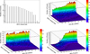 |
Fig. 5 Number of PWR-MOx missed loadings at the end of scenario (t = 100 years). The figure up left is the distribution. Plots up right, bottom left and bottom right are respectively their distribution according to the PWR-UOx Burn-Up, the PWR-MOx Burn-Up and the PWR-MOx thermal power fraction. |
4.4 Thermal power evolution
In this section, the impact on missed load on thermal power deviation is investigated. Indeed, comparison between outputs has meaning if the energy produced in scenarios are identical. Figure 6 represents thermal power and cumulated thermal energy according to the time for all the simulations. On the plot related to the power, green points represent simulations for which PWR MOx have zero missed fuel loading.
Also, an artifact appears between t = 20 years and t = 25 years showing that thermal power is not completely constant in the simulation. This is due to the option of leaving the PWR-UOx ends its irradiation cycle time before having a thermal power reduced by the PWR-MOx thermal power, which starts in all case at t = 20 years. The effect of this artifact could be calculated from the thermal energy plot. The thermal energy deviation at the end of scenario for simulations without missed loadings is closed to 1. The effect of the artifact is then considered as negligible.
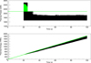 |
Fig. 6 Thermal power and cumulated energy according to the time for all the simulations. The green points represent a selection in which there is no missed loadings for the PWR MOx. |
5 Plutonium production analysis
5.1 Plutonium production dependency
In this section, the plutonium production is assessed in detail according most impacting input variables identified in Section 4.2. The plutonium total mass evolution for all the runs is represented in Figure 7 superimposed by the runs without PWR-MOx missed loadings.
To get plutonium production main drivers without any bias, only runs with no missed loadings at the end of scenario are taken into account. Figure 8 shows the plutonium inventory at the end of scenario (t = 100 years) according to most important input variables which are PWR UOx Burn-Up and PWR-MOx thermal power fraction.
The plot at the top left represents plutonium total mass in the fleet after 100 years of operation. It shows that plutonium mass production decreases with the increase of the PWR-UOx Burn-Up. This is an effect due to the decrease of the plutonium slope production in a PWR-UOx with the Burn-Up. The top right plot shows the total plutonium at the end of scenario according the PWR-MOx power fraction. The global trend shows a well known effect, which is the plutonium partial incineration in the PWR-MOx reactor. The bottom 3D plot clearly shows that the plutonium mass at the end of scenario has a small variability if PWR-UOx Burn-Up and PWR-MOx power fraction are fixed. As expected in the section dedicated to Sobol’ indices calculation, this suggests the plutonium variance could be mainly explained by those two input variables, as expected by Sobol’ indices for plutonium.
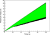 |
Fig. 7 Plutonium mass evolution for all runs in black and for runs without reactor missed loadings in green. |
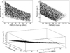 |
Fig. 8 Plutonium mass at the end of scenario according to PWR-UOx Burn-Up (top left) and PWR-MOx thermal power fraction (top right). The plot at the bottom represents a 3D visualization. |
5.2 Equilibrium condition in stockpile
Optimal conditions for recycling the plutonium in PWR-MOx fuel has been also investigated. The plutonium stockpile is fed by the spent PWR-UOx fuel and provides plutonium to the PWR-MOx fuel. The equilibrium conditions, which supposes that plutonium is available during all the scenario and does not increase is given by:
-
no PWR-MOx missed loadings during the run;
-
plutonium mass at the end of scenario is lower than 3.5 tons, which corresponds to the plutonium maximum mass at the PWR-MOx first loading (t = 20 years).
Figure 9 shows plutonium mass evolution in the dedicated stockpile without (black dots) and with the two conditions written above (green dots). Plutonium equilibrium conditions has been applied to extract equilibrium condition according to PWR-UOx Burn-Up and PWR-MOx fraction. A solution appears and could be quantified by data provided in Table 5.
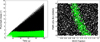 |
Fig. 9 Plutonium mass evolution in available stockpile (left, black dots) with runs with plutonium closed to equilibrium (left, green dots). Design of experiment according to MOx Fraction and UOx BU (right, black dots) and plutonium equilibrium condition sub-space (right, green dots). |
Indicative solution space for plutonium equilibrium in the PWR-UOx spent fuel stockpile.
5.3 Plutonium fissile fraction at beginning of cycles
In this section, the impact of input variables on the plutonium quality loaded in the PWR-MOx fuel is assessed. For this purpose, the plutonium fissile fraction Puff at B.O.C. is calculated as the ratio between 239Pu and 241Pu mass on the total plutonium mass. Figure 10 shows Puff distribution for LIFO (top) and FIFO (bottom) strategies which spreads respectively from 0.63 to 0.73 and from 0.61 to 0.71. For the two plots represented, data are selected for runs without PWR-MOx missed loadings and for a time higher that 20 years (after the PWR-MOx start).
As a preliminary remark, it is observed that the fuel strategy has a small impact on the plutonium fissile content at PWR-MOx B.O.C. Nevertheless, the LIFO (resp. FIFO) strategy leads to a higher (resp. lower) fissile content. A LIFO strategy induces small cooling time for available plutonium and a small impact of the 241Pu decay. Plots of Figure 10 also show the importance of PWR-UOx Burn-Up in the plutonium fissile content. The smaller the Burn-Up is, the higher the fissile content of fresh fuel is. Indeed, during PWR-UOx irradiation, the 239Pu is the precursor to the production of other important plutonium isotopes. Increasing the PWR-UOx Burn-Up leads to a higher fraction of other isotopes in the plutonium vector. For each distribution, the average value has been extracted and reported in Table 6.
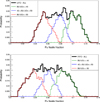 |
Fig. 10 Distribution of plutonium fissile content at PWR-MOx beginning of cycle for LIFO strategy at the top and FIFO strategy at bottom. Plots show also the contribution of Burn-Up ranges in the plutonium fissile content distribution. |
Average value of plutonium fissile fraction distributions according to applied conditions.
6 Minor actinides inventory evolution
This section aims to present MA evolution drivers in the simulated fleet. According to Table 3, MA production variability, dominated by the americium production, is explained by almost all the input variable, unlike plutonium production variability which mainly depends on two variables.
6.1 Neptunium production
The Neptunium production is mainly impacted by the PWR-UOx Burn-Up and the PWR-MOx fraction, as shown in Figure 11 bottom 3D view, and as it was expected by Sobol’ indices of Table 3.
The increase of the neptunium production according to the PWR-UOx Burn-Up could be understood from its production pathways. The neptunium element is represented mainly by the isotope 237Np which is mainly produced by those two pathways:
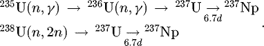 (6)
(6)
We consider here that the production of 237Np from 241Am decay is a small contribution. At beginning of PWR-UOx cycle, as there is no 236U, 237Np is produced mainly via (n, 2n) reaction on 238U. After a small irradiation time (around 3 GWd/t), the neutron capture rate on 236U is getting above the (n, 2n) reaction on 238U and becomes the main pathway for the 237Np production. The 237Np production is then in almost all the irradiation proportional to the 236U mass, which increase during the irradiation. This explains the fact that the 237Np production slope increases during irradiation in the considered Burn-Up range and justify the 237Np dependency with the PWR-UOx Burn-Up.
The neptunium production decreases slowly with the PWR-MOx Burn-Up. The 237Np evolution is almost linear in a PWR-MOx fuel and quite negligible compared to production in PWR-UOx. The PWR-MOx fraction does not directly affects the 237Np production but decreases the PWR-UOx produced energy which decreases the 237Np mass at the end of scenario.
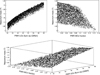 |
Fig. 11 Neptunium mass at the end of scenario according to PWR-UOx Burn-Up (top left) and PWR-MOx thermal power fraction (top right). The plot at the bottom represents a 3D visualization. |
6.2 Americium production
The americium production Sobol’ indices analysis is more complex. 241Am production is mainly driven by the PWR-UOx Burn-Up even though its production in reactor is small. This is due to the strong correlation between the 241Am and the 241Pu production, as showed in Figure 12. As the 241Pu production is strongly correlated with the PWR-UOx Burn-Up, the 241Am production is also impacted.
A relevant observation is the fuel strategy effect on Sobol’ indices. Indeed, the spent UOx fuel cooling time has an important impact on 241Am production in LiFo fuel strategies but not in FiFo. This can be interpreted by seeing the available isotopic vector in the stockpile as a stack (see Fig. 13). Whatever the cooling time is, the older fuel in the stack is always the same, provided the stockpile is not empty, which is the case since PWR-MOx missed loadings is not allowed. On the other hand, the latest isotopic vector chosen in the case of LiFo strategy will depend on the cooling time. As the 241Am is produced mainly by the 241Pu decay, with a half-life of 14.35 years, this effect is specifically important.
Also, the 241Am mass at the end of scenario depends on the PWR-MOx fraction. Indeed, the average 241Am mass are 2.2 and 2.4 tons respectively for LiFo and FiFo fuel strategies. The 241Pu produced mass in PWR-MOx (cf. Fig. 12 on the right) per reactor cycle shows that the LiFo strategy produces less 241Pu than the FiFo strategy. The FiFo strategy means a smaller 241Pu amount in the fuel, what induces a higher production rate in the reactor during the irradiation. More 241Pu produced in the PWR-MOx reactor leads thus to more 241Am produced at the end of scenario.
Concerning 243Am, the main driver is the PWR-MOx fraction. 243Am is mainly generated by neutron capture on 242Pu followed by a beta decay. As increasing the PWR-MOx fraction increases the 242Pu amount, this explains the strong impact of the PWR-MOx fraction on the 243Am production.
Second order indices are important for the MA in LiFo strategy. Interaction between UOx Burn-Up and MOx fraction is 0.19 and interaction between UOx cooling time and MOx fraction is 0.12. The sum of first and second indices are closed to the total indices, which suggests three variable interaction is negligible. For MA in LiFo strategy, interactions are driven by the MOx fraction. This can be interpreted as the effect of PWR-MOx deployment on other input variable. The UOx cooling time has no effect on MA production if MOx fraction is very small. The UOx Burn-Up effect is maximum for small MOx fraction. The MA production in FiFo strategy is characterized by a second order indices between UOx Burn-Up and MOx fraction close to 0.16, which is the exact difference between first and total indices.
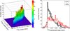 |
Fig. 12 241Am and 241Pu masses distribution at the end of scenario on the left. 241Pu produced mass during the first PWR-MOx cycle. |
 |
Fig. 13 Schematic representation showing the impact of the fuel strategy on the isotopic vector chosen for building the PWR-MOx fresh fuel. The colored parts (red and green) show which fraction of the stockpile is used for LiFo and FiFo strategy. |
6.3 Curium production
According to Table 3, curium production strongly depends on PWR-MOx fraction. Smallest dependency with PWR-UOx and PWR-MOx Burn-Up is also observed. This is justified by the curium production that is induced by neutron capture on plutonium isotopes. Figure 14 represents the curium mass at the end of scenario. The left plot shows how the curium production increases with the PWR-MOx fraction. The plot on the right shows the strong correlation between curium production and plutonium inventory at the end of scenario. An interpretation is that less plutonium means more nuclear reactions among which neutron captures responsible of curium production.
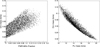 |
Fig. 14 Curium mass dependency with PWR-MOx fraction (left) and correlation with plutonium mass (right). |
7 Conclusions
Fuel cycle simulators are used worldwide to provide scientific assessment to fuel cycle future strategies. Those tools help understanding the fuel cycle physics and determining the most impacting drivers at the cycle scale. This paper has presented an innovative methodology based on GSA applied to nuclear fuel cycle simulation. In this new framework, operational assumptions of scenarios, such as reactor burn-up, deployment date and so on, could be sampled as input variable of the model represented by the fuel cycle simulator. The CLASS code has been used for performing this analysis. The methodology has been applied to a simple scenario calculation composed by a PWR-UOx and a PWR-MOx fuel operated during 100 years. A preliminary analysis of the sample leads to an important model improvement related to the fresh fuel determination algorithm. Sobol’ indices have been estimated for input variables and for a wide range of output data. Main drivers could be determined and PWR-UOx Burn-Up as the PWR-MOx fraction are the most impactive variables for a majority of tested output data. The variability of plutonium production can be explained with those two variables. MA production is more complex, since pool cooling time and PWR-MOx Burn-Up could have a non-negligible impact. This innovative methodology can be applied to any fuel cycle simulator. Nevertheless, small limitations appears. If the computing time and the RAM utilization are not problematic, the output data storage can be a drawback, especially for testing model parameters or uncertainty propagation on an output. In those specific cases, a design of experiment should be run several times and storage limitations could appear. A solution could be to impose an output data selection during the run in order to select only needed information. A lot of benchmarks was dedicated to compare fuel cycle tools inventories estimation for simple or complex scenarios. The presented methodology could provide an interesting prospective direction for fuel cycle benchmark. Indeed, if fuel cycle tools produce different absolute results, they may produce similar sensitivity to input variables. This could help to redefine application domain for fuel cycle simulators, more adapted to provide appropriate answers. This methodology for fuel cycle studies has to be tested on precise fleet including a high number of reactors. Also, a lot of output observable could be tested according to the problematic, such as cost of electricity optimisation, natural uranium consumption and so on.
Author contribution statement
The work presented in this paper is mainly produced by a collaboration in the framework of a NEEDS project. N. Thiollière has designed and run the simulations, analyzed the results and written the article. J.B. Clavel, F. Courtin, X. Doligez, M. Ernoult, Z. Issoufou and G. Krivtchik have developed the methodology based on Global Sensitivity Analysis applied for fuel cycle simulators. B. Leniau and B. Mouginot are the main developers of the CLASS tool used in this work. A. Bidaud, S. David, V. Lebrin, C. Perigois, Y. Richet and A. Somaini are or was members of the collaboration.
Acknowledgments
We would like to express our gratitude to the NEEDS program of the Energy Unit of the CNRS (Centre National de la Recherche Scientifique) for the financial support. We also thank Dr Baptiste Mouginot, for his major work as the main developer of the fuel cycle simulator CLASS and Dr Baptiste Leniau for his great work on neutron data predictor implementation.
References
- F. Courtin, Study of plutonium incineration in PWR loaded with MOx on enriched uranium support with the fuel cycle simulator CLASS, Theses, Ecole nationale supérieure Mines-Télécom Atlantique, 2017, https://tel.archives-ouvertes.fr/tel-01668610 [Google Scholar]
- Direction de l’Energie Nucléaire du CEA, Loi du 28 juin 2006 relative à la gestion durable des matières et des déchets radioactifs: bilan des recherches conduites sur la séparation-transmutation des éléments radioactifs à vie longue et sur le développement de réacteurs nucléaires de nouvelle génération, Tome 1: La gestion durable des matières radioactives avec les réacteurs de quatrième génération, 2012 [Google Scholar]
- M. Tiphine, C. Coquelet-Pascal, G. Krivtchik, R. Eschbach, C. Chabert, G.C.M. Caron-Charles, G. Senentz, L.V. den Durpel, C. Garzenne, F. Laugier, Simulations of progressive potential scenarios of pu multirecycling in SFR and associated phaseout in the french nuclear power fleet, in Global 2015 Proceedings (2015) [Google Scholar]
- G.V. den Eynde, V. Romanello, F. Martin-Fuertes, C. Zimmerman, B. Lewin, A. Van Heek, Status of the EC-FP7 Project ARCAS: Comparing the economics of accelerator-driven systems and fast reactors as minor actinide burners, in Actinide and Fission Product Partitioning and Transmutation, OECD/NEA (Paris, France, 2013), pp. 301–313 [Google Scholar]
- C. Coquelet-Pascal, M. Tiphine, G. Krivtchik, D. Freynet, C. Cany, R. Eschbach, C. Chabert, Nucl. Technol. 192, 91–110 (2015) [CrossRef] [Google Scholar]
- K.D. Huff, M.J. Gidden, R.W. Carlsen, R.R. Flanagan, M.B. McGarry, A.C. Opotowsky, E.A. Schneider, A.M. Scopatz, P.P. Wilson, Adv. Eng. Softw. 94, 46–59 (2016) [CrossRef] [Google Scholar]
- M.B. McGarry, D. Buys, C. Hoffman, B. Mouginot, P.P.H. Wilson, State-level decision-making in cyclus to assess multilateral enrichment, in INMM 58th Annual Meeting (Indian Wells, USA, 2017) [Google Scholar]
- M. Göttsche, B. Mouginot, An integrated nuclear archaeology approach to reconstruct fissile material production histories, in 39th ESARDA Symposion (Germany, 2017) [Google Scholar]
- J.J. Jacobson, A.M. Yacout, G.E. Matthern, S.J. Piet, D.E. Shropshire, R.F. Jeffers, T. Schweitzer, Nucl. Technol. 172, 157–178 (2010) [CrossRef] [Google Scholar]
- F. Âlvarez-Velarde, E. Gonzàlez-Romero, I.M. Rodriguez, Ann. Nucl. Energy 73, 175–188 (2014) [CrossRef] [Google Scholar]
- L. Van Den Durpel, in Proceedings of the 20th Pacific Basin Nuclear Conference, 2017, edited by H. Jiang (Springer Singapore, 2017), pp. 463–476 [CrossRef] [Google Scholar]
- G. Krivtchik, Thesis, Université de Grenoble, 2014, https://tel.archives-ouvertes.fr/tel-01131207 [Google Scholar]
- B. Hyland, D. Wojtaszek, C. Coquelet-Pascal, D. Freynet, F. Alvarez-Velarde, M. Garciac, B. Dixon, F. Gabrielli, B. Vezzoni, G. Glinatsis, K. Ono, A. Ohtaki, E. Malambu, B. Carlier, S. Cornet, The Effects of the Uncertainty of Input Parameters on Nuclear Fuel Cycle Scenario Studies, Technical Report, Nuclear Energy Agency of the OECD (NEA), 2015 [Google Scholar]
- A. Baker, R. Ross, Comparison of the value of plutonium and uranium isotopes in fast reactors, in USAEC, Breeding, Economics, and Safety in Large Fast Breeder Reactors (Argonne National Laboratory, Illinois, 1963), pp. 329–365 [Google Scholar]
- B. Leniau, B. Mouginot, N. Thiollière, X. Doligez, A. Bidaud, F. Courtin, M. Ernoult, S. David, Ann. Nucl. Energy 81, 125–133 (2015) [CrossRef] [Google Scholar]
- A. Somaini, S. David, X. Doligez, A. Zakari-Issoufou, A. Bidaud, N. Cappelan, O. Meplan, A. Nuttin, P. Prevot, F. Courtin, B. Leniau, B. Mouginot, N. Thiolliere, The impact of reactor model simplification for fuel evolution: a bias quantification for fuel cycle dynamic simulations, in 2016 International Congress on Advances in Nuclear Power Plants (ICAPP 2016) (San Francisco, United States, 2016), pp. 1045–1053, http://hal.in2p3.fr/in2p3-01346740 [Google Scholar]
- A. Saltelli, S. Tarantola, F. Campolongo, M. Ratto, Sensitivity Analysis in Practice: A Guide to Assessing Scientific Models (Halsted Press, New York, NY, USA, 2004) [Google Scholar]
- A. Saltelli, K. Chan, E.M. Scott, Sensitivity Analysis (Wiley, 2009) https://books.google.fr/books?id=gOcePwAACAAJ [Google Scholar]
- A. Saltelli, P. Annoni, I. Azzini, F. Campolongo, M. Ratto, S. Tarantola, Comput. Phys. Commun. 181, 259–270 (2010) [CrossRef] [Google Scholar]
- J. Jacques, Theses, Université Joseph-Fourier - Grenoble I, 2005, https://tel.archives-ouvertes.fr/tel-00011169 (2011) [Google Scholar]
- R. Brun, F. Rademakers, Nucl. Instrum. Methods A389, 81–86 (1997) [CrossRef] [Google Scholar]
- M.D. McKay, R.J. Beckman, W.J. Conover, Technometrics 21, 239–245 (1979) [Google Scholar]
- B. Mouginot, B. Leniau, N. Thiollère, M. Ernoult, S. David, X. Doligez, A. Bidaud, O. Meplan, R. Montesanto, G. Bellot, J. Clavel, I. Duhamel, E. Letang, J. Miss, Core library for advanced scenario simulation, CLASS: principle and application, in PHYSOR 2014–The Role of Reactor Physics toward a Sustainable Future (2014) [Google Scholar]
- F. Casella, A. Bidaud, N. Thiollière, Economic Module development for the Fuel Cycle Simulation tool CLASS and its application on the Brazil-Argentinean scenario,Master’s thesis, Laboratoire de Physique Subatomique et de Cosmologie de Grenoble, 2016 [Google Scholar]
- A. Hoecker, P. Speckmayer, J. Stelzer, J. Therhaag, E. Von Toerne, H. Voss, PoS ACAT 040 (2007) [Google Scholar]
- A.-A. Zakari-Issoufou, X. Doligez, A. Somaini, Q. Hoarau, S. David, S. Bouneau, F. Courtin, B. Leniau, N. Thiollière, B. Mouginot, A. Bidaud, N. Capellan, O. Meplan, A. Nuttin, Ann. Nucl. Energy 102, 220–230 (2017) [CrossRef] [Google Scholar]
- A. Janon, T. Klein, A. Lagnoux-Renaudie, M. Nodet, C. Prieur, ESAIM: Probab. Stat. 18, 342–364 (2014) [CrossRef] [Google Scholar]
- G. Pujol, B. Iooss, A.J. with contributions from Khalid Boumhaout, S.D. Veiga, T. Delage, J. Fruth, L. Gilquin, J. Guillaume, L.L. Gratiet, P. Lemaitre, B.L. Nelson, F. Monari, R. Oomen, B. Ramos, O. Roustant, E. Song, J. Staum, T. Touati, F. Weber, Sensitivity: Global Sensitivity Analysis of Model Outputs (2017), http://CRAN.R-project.org/package=sensitivity, r package version 1.14.0 [Google Scholar]
- R Core Team, R: A Language and Environment for Statistical Computing (R Foundation for Statistical Computing, Vienna, Austria, 2015), https://www.R-project.org/ [Google Scholar]
Commissariat à l’énergie atomique et aux énergies alternatives.
Centro de Investigaciones Energèticas, Medioambientales y Tecnològicas.
Centre National de la Recherche Scientifique.
Institut National de Physique Nucléaire et de Physique des Particules.
Institut de Radioprotection et de Sûreté Nucléaire.
Cite this article as: Nicolas Thiollière, Jean-Baptiste Clavel, Fanny Courtin, Xavier Doligez, Marc Ernoult, Zakari Issoufou, Guillaume Krivtchik, Baptiste Leniau, Baptiste Mouginot, Adrien Bidaud, Sylvain David, Victor Lebrin, Carole Perigois, Yann Richet, Alice Somaini, A methodology for performing sensitivity analysis in dynamic fuel cycle simulation studies applied to a PWR fleet simulated with the CLASS tool, EPJ Nuclear Sci. Technol. 4, 13 (2018)
All Tables
Sobol’ first order and total indices estimation. Four input variables are in column. Fuel strategy is specified if there is more than 5% difference between indices. The mention "All" means there is no difference between fuel strategies. Only indices higher than 0.05 are represented. PWR Burn-Up are mentioned (UOx BU and MOx BU), as the PWR-MOx thermal power fraction (Fr. MOx). CT UOx is the spent UOx cooling time.
Indicative solution space for plutonium equilibrium in the PWR-UOx spent fuel stockpile.
Average value of plutonium fissile fraction distributions according to applied conditions.
All Figures
|
Fig. 1 Schematic representation of fuel cycle simulations. |
| In the text | |
|
Fig. 2 Input and output data tree structure. |
| In the text | |
|
Fig. 3 Schematic principle of the CLASS library. |
| In the text | |
|
Fig. 4 Corrupted events according to PWR-UOx Burn-Up and PWR-MOx thermal power fraction in the total thermal power. This plot has been obtained with the previous CLASS version before the improvement of the FLM. |
| In the text | |
|
Fig. 5 Number of PWR-MOx missed loadings at the end of scenario (t = 100 years). The figure up left is the distribution. Plots up right, bottom left and bottom right are respectively their distribution according to the PWR-UOx Burn-Up, the PWR-MOx Burn-Up and the PWR-MOx thermal power fraction. |
| In the text | |
|
Fig. 6 Thermal power and cumulated energy according to the time for all the simulations. The green points represent a selection in which there is no missed loadings for the PWR MOx. |
| In the text | |
|
Fig. 7 Plutonium mass evolution for all runs in black and for runs without reactor missed loadings in green. |
| In the text | |
|
Fig. 8 Plutonium mass at the end of scenario according to PWR-UOx Burn-Up (top left) and PWR-MOx thermal power fraction (top right). The plot at the bottom represents a 3D visualization. |
| In the text | |
|
Fig. 9 Plutonium mass evolution in available stockpile (left, black dots) with runs with plutonium closed to equilibrium (left, green dots). Design of experiment according to MOx Fraction and UOx BU (right, black dots) and plutonium equilibrium condition sub-space (right, green dots). |
| In the text | |
|
Fig. 10 Distribution of plutonium fissile content at PWR-MOx beginning of cycle for LIFO strategy at the top and FIFO strategy at bottom. Plots show also the contribution of Burn-Up ranges in the plutonium fissile content distribution. |
| In the text | |
|
Fig. 11 Neptunium mass at the end of scenario according to PWR-UOx Burn-Up (top left) and PWR-MOx thermal power fraction (top right). The plot at the bottom represents a 3D visualization. |
| In the text | |
|
Fig. 12 241Am and 241Pu masses distribution at the end of scenario on the left. 241Pu produced mass during the first PWR-MOx cycle. |
| In the text | |
|
Fig. 13 Schematic representation showing the impact of the fuel strategy on the isotopic vector chosen for building the PWR-MOx fresh fuel. The colored parts (red and green) show which fraction of the stockpile is used for LiFo and FiFo strategy. |
| In the text | |
|
Fig. 14 Curium mass dependency with PWR-MOx fraction (left) and correlation with plutonium mass (right). |
| In the text | |
Current usage metrics show cumulative count of Article Views (full-text article views including HTML views, PDF and ePub downloads, according to the available data) and Abstracts Views on Vision4Press platform.
Data correspond to usage on the plateform after 2015. The current usage metrics is available 48-96 hours after online publication and is updated daily on week days.
Initial download of the metrics may take a while.