| Issue |
EPJ Nuclear Sci. Technol.
Volume 12, 2026
|
|
|---|---|---|
| Article Number | 8 | |
| Number of page(s) | 16 | |
| DOI | https://doi.org/10.1051/epjn/2025079 | |
| Published online | 04 March 2026 | |
https://doi.org/10.1051/epjn/2025079
Regular Article
Extension of the turbulent heat flux modelling in OpenFOAM for improved simulation of liquid metal flows
Gesellschaft für Anlagen- und Reaktorsicherheit (GRS) gGmbH, Boltzmannstr. 14, 85748 Garching, Germany
* e-mail: This email address is being protected from spambots. You need JavaScript enabled to view it.
Received:
5
August
2025
Received in final form:
5
December
2025
Accepted:
9
December
2025
Published online: 4 March 2026
Abstract
Turbulent heat transfer is a fundamentally complex physical process that has challenged turbulence modellers for many years. A full differential second-moment closure model provides a solid foundation for the derivation of the simpler Algebraic Heat Flux Model (AHFM), which retains the primary production terms that represent the underlying physical mechanisms driving the turbulent heat flux. This allows for accurate modelling of natural and mixed convection flows, which becomes particularly evident in advanced nuclear reactor applications with low Prandtl number coolants. In the present work, an AHFM model was implemented in the open-source code OpenFOAM, and was first verified using a simple channel test case. In the next step, the implementation was validated against Direct Numerical Simulation (DNS) data of a Rayleigh–Bénard convection case. The latter was based on simple geometry with natural convection of a low-Prandtl-number fluid, being of particular importance for Generation IV reactors using liquid metal coolants. The comparison of the generated numerical results with DNS data demonstrated the improvements in the prediction of turbulent heat flux in low-Prandtl number fluids with the new model.
© H. Mistry et al., Published by EDP Sciences, 2026
 This is an Open Access article distributed under the terms of the Creative Commons Attribution License (https://creativecommons.org/licenses/by/4.0), which permits unrestricted use, distribution, and reproduction in any medium, provided the original work is properly cited.
1. Introduction
As the global demand for sustainable and high-efficiency energy sources increases, advanced nuclear reactor designs are receiving renewed interest. Among these, Liquid Metal Fast Reactors (LMFRs)–such as the Sodium Fast Reactor (SFR) and the Lead Fast Reactor (LFR)–stand out as promising Generation IV nuclear systems due to their excellent neutron economy, closed fuel cycle potential, and superior thermal properties [1, 2]. The use of liquid metals as primary coolants in these reactors offers several advantages, including high thermal conductivity, low neutron moderation, and high boiling points, enabling efficient heat removal at near-atmospheric pressure [3].
However, despite these thermophysical advantages, the prediction of the turbulent heat transfer in LMFRs remains a significant challenge, primarily due to the very low-Prandtl numbers of liquid metals–typically ranging between 0.001 and 0.025 under reactor operating conditions [4]. In such regimes, the disparity between thermal and momentum diffusivities leads to thick thermal boundary layers, anisotropic turbulence, and heat transfer mechanisms that are not well captured by conventional models designed for unity-Pr fluids like water or air [5]. Due to the high thermal conductivity and low viscosity of lead, sodium, etc., the near-wall temperature shear layers differ significantly from the momentum boundary layers. This can lead to inadequate heat flux, temperature and velocity profiles in analyses with heat transfer from or to the wall. This is especially critical in transition regimes between convection-dominated and conduction flow, often encountered in reactor cores and internal components.
Conventional Computational Fluid Dynamics (CFD) simulations of turbulent heat transfer commonly rely on the Simple Gradient Diffusion Hypothesis (SGDH), which assumes a linear relationship between the turbulent heat flux and the mean temperature gradient via a turbulent Prandtl number [6]. While this approach yields acceptable predictions for engineering applications involving unity-Prandtl fluids, its limitations become increasingly apparent in low Prandtl number flows, where the assumptions of isotropy and flux-gradient alignment no longer hold [7–9]. These limitations are particularly significant in mixed and natural convection regimes, as noted in the OECD/NEA benchmark studies [4] and highlighted in [10].
Generally, the two equations model is based on eddy viscosity, eddy diffusivity and the Reynolds analogy [11]. In such models, the turbulent momentum transport and the turbulent heat transport are assumed to be proportional [12], which is not true for liquid metal flows, which exhibit higher thermal diffusivity compared to the molecular viscosity [13, 14]. To overcome the limitations of eddy diffusivity-based models, Algebraic Heat Flux Models (AHFMs) have emerged as an alternative that provides more physically accurate results. AHFMs are derived from second-order moment closures and account for anisotropic turbulence effects, mean velocity gradients, buoyancy, and other non-local interactions [15, 16]. One notable formulation was proposed by Kenjereš [17], incorporating these terms in an algebraic frame-work suitable for engineering CFD. However, the original model coefficients were calibrated primarily for flows with Pr ≈ 1, limiting their application to liquid metal scenarios.
Further implementation and validation of AHFM model is shown by Shams [18] for commercial software STAR-CCM+. An important step forward was taken by Shams [9], who recalibrated the AHFM coefficients for forced convection at low Prandtl numbers. Their formulation introduced a logarithmic dependency on the global Reynolds and Prandtl numbers. While this extension broadened the model’s theoretical applicability, it also introduced a significant limitation: the need for defining a global Reynolds number and characteristic length scale, which may not be well-defined or spatially consistent in complex geometries such as reactor cores, heat exchangers, or flow around fuel assemblies. Moreover, the requirement for a priori knowledge of bulk flow quantities poses challenges in transient simulations, where these quantities evolve over time [9].
Another attempt to improve the simulation of low-Prandtl number fluids with the help of AHFM can be found in the work of Habiyaremye [19]. There, a new AHFM formulation is presented, in which a local turbulent Reynolds number and the fluid’s molecular Prandtl number are used to calculate the model’s coefficient that is associated with forced convection. The coefficient was calibrated in two different forced convection cases by minimizing the error in the temperature profiles compared to reference DNS data at low Prandtl numbers (i.e. Pr < 0.2). Two additional forced convection cases were used to validate the new coefficient formulation. It was shown that in all geometries, the new formulation performs better than the commonly used SGDH at low Prandtl numbers.
To improve the modelling of the turbulent heat flux in liquid metal flows, Manservisi [20] decided to use a four parameters k − ε − kθ − εθ turbulence model, which was then tested for the simulation of basic cases. The investigation of the heat transfer models based on variable turbulent Prandtl number for liquid metal flows is performed by using both momentum and energy transport turbulence equations.
Further attempt to deal with turbulent heat flux in liquid metal flows was done at KIT, Germany. It is based on look-up tables and the determination of a local variable turbulent Prandtl number from DNS data. The implementation of this approach depends on the local Prandtl number, the global Reynolds number, and the y+ value, which is estimated from a pre-calculation. Although, this approach is robust and performed reasonably well for pipe and rod bundle flows, buoyant, natural convection flows could not be predicted well, and the intermittency effects were not considered. The advantages of the look-up tables are robustness and the fact that additional equations are not required. The drawbacks are mainly related to the applied isotropic Reynolds analogy and the dependency of the implementation on the wall spacing.
In order to be able to accurately map the behaviour of fluids with a low Prandtl number with OpenFOAM, first implementation at GRS of an AHFM turbulence model in OpenFOAM was done within the RS1547 [21] research project. The available OpenFOAM incompressible non-linear turbulence model LienCubicKE [22, 23] was extended with an AHFM implementation called LienCubicKEAHFM and released within OpenFOAM Foundation Version 6. Also, a special solver (buoyantBoussinesqPimpleFoamAHFM) was developed for simulations, in which the calculation of the buoyancy is based on the Boussinesq approximation. However, this specific solver has not been further pursued after OpenFOAM Version 7, which was released in 2019 [24]. Its successor, the buoyantPimpleFoam solver, does not solve the transport equation for the temperature, but rather for the energy. In addition to that, OpenFOAM Foundation has made massive changes to the code structure, which lead to a high implementation effort of the AHFM in the new version, as well as duplication of some Open-FOAM internal libraries. Therefore, another solution was necessary.
In the present work, the developed turbulent heat flux model is extended on the basis of the existing material libraries and made usable with the basic solvers (fluid and incompressible Fluid) [25]. The turbulence model is formulated to be used for compressible and incompressible flows. In addition, a new turbulence model based on Non-Linear Eddy Viscosity model (NLEVM) has been implemented. The developments were implemented with the kind support of HZDR in their NUSAR-RCS code that is based on OpenFOAM Foundation version 12-s.1 [26]. The new development is verified and then validated against DNS data for natural convection in a slender geometry.
2. AHFM implementation in OpenFOAM
This section provides short details on the turbulent heat flux theory as well as on the AHFM implementation strategy.
2.1. Turbulent heat flux
The Reynolds-averaged momentum and energy equations with turbulent flows for most industrial application are defined as [27]:
 (1)
(1)
 (2)
(2)
where,  represents the material derivative, Fi is the body force per unit mass, qi is the internal energy source, and Cp is heat capacity of fluid. In these equations,
  denotes the turbulent momentum flux, while
  is turbulent heat flux correlation with fluctuating velocity–temperature. To obtain an adequate closure of the mathematical system, models are added to close the nonlinear terms.
The traditional definition of the turbulent heat flux in the energy equation is based on the Boussinesq assumption, which assumes that the heat flux is aligned with the temperature gradient and scaled by the turbulent eddy viscosity. This approximation fails in the case of a flow regime that deviates from the energy equilibrium, such as a buoyancy-dominant flow. Consequently, the primary objective of a heat flux model should be to deliver accurate and reliable results across all types of flow regimes [27]. With such a limitation, sophisticated turbulent heat flux modelling approaches have to be employed.
2.2. Algebraic heat flux model
Several AHFMs have been developed within the European THINS [28] and SESAME projects [29] such as an explicit and implicit formulation. In the explicit formulation, the turbulent heat flux is determined using the gradient hypothesis combined with the eddy diffusivity concept. This involves the definition of suitable turbulence timescales, which results in the development of four-parameter turbulence models [20]. Due to its isotropic nature, this approach has some limitations and requires further validation. In the implicit approach, the turbulent heat flux is obtained by directly solving a nonlinear algebraic equation derived from the transport equation for turbulent heat flux, using an algebraic solution method [17]. This formulation is a function of Reynolds stress anisotropy and temperature variance, for which an additional transport equation is solved. Accordingly, this implicit formulation is implemented in this study as described in [17].
The performance of the AHFM model is closely related to the correct approximation of the turbulent behaviour near the wall, and therefore, requires a low Reynolds number turbulence model. In general, the unknown Reynolds stress tensor or turbulent momentum flux  is assumed to obey a linear constitutive relation based on the mean strain rate [15, 27].
 (3)
(3)
The turbulent heat flux  is commonly represented by the simple eddy-diffusivity model, which is based on the Reynolds analogy defined as:
 (4)
(4)
where, k is the turbulent kinetic energy, νt is the eddy viscosity, δij is the Kronecker delta, αt is the turbulent thermal diffusivity, and Prt is the turbulent Prandtl number (constant value of 0.9) [27].
In AHFM, the algebraic equation of turbulent heat flux proposed by Kenjereš [17] is implicitly solved using an algebraic method,
 (5)
(5)
where, ε is turbulent kinetic energy dissipation rate, aij is the Reynolds stress anisotropy tensor defined as  . The terms appearing in equation (5) with Ct1 and Ct2 model coefficients describe the production of turbulent heat flux due to non-uniform mean temperature and velocity field, respectively. The term with Ct3 model coefficient is amplification of turbulence fluctuations due to the effect of buoyancy, and the last term with Ct4 model coefficient is redistribution of turbulent heat flux due to anisotropic turbulence [15, 30]. On the other hand, the gravitational acceleration gi, the thermal expansion coefficient β, and the turbulent fluctuations in temperature as temperature variance
  [9, 18], which are modelled with a separate field equation, are used to solve the turbulent heat flow
  .
.
 (6)
(6)
where, κ is thermal conductivity of fluid, μt is the dynamic turbulent viscosity,  is the production of temperature variance, and εθ is its dissipation rate. The most generic approach for solving the above equation is when the dissipation rate εθ is solved with an additional transport equation. Velocity and the thermal fields in liquid metal flows are characterized by different length and time-scales. In the thermal boundary layer, the time-scales differ up to two orders of magnitude [27]. As a result, this type of modelling contains more than two free parameters including turbulent time-scales. Thus, most models stick with a simpler approach and assume a constant thermal
  to mechanical time-scale (τm = k/ε) ratio R:
 (7)
(7)
The complete AHFM model is expressed in three-equation terms of k, ε, and  . The k and ε turbulence equations will be discussed in following section.
2.3. Turbulence modelling
As mentioned earlier, the Boussinesq linear stress-strain relation is unable to accurately simulate anisotropic turbulence in real-world flow scenarios, because it ignores variations in the normal stresses. By taking into account non-linear correlations between Reynolds stresses and strain rates, nonlinear models attempt to overcome this limitation. These NLEVMs belong to an intermediate class of turbulence models. In these, the Reynolds stress is explicitly expressed algebraically in terms of vorticity tensors and the strain rate. Depending on the accuracy level, theoretically functional term forms as quadratic or cubic model. In OpenFOAM, these terms have a simplified general stress-strain formulation following [23]:
![Mathematical equation: $$ \begin{aligned} a_{ij}&=- 2{C_{\mu }f_{\mu }S}_{ij}+\bigg [\beta _{1}\left( S_{ik}S_{kj}-\frac{1}{3}S_{lk}S_{lk}\delta _{ij} \right)\nonumber \\&\quad +\beta _{2}\left({S}_{ik}\mathrm{\Omega }_{kj}-\mathrm{\Omega }_{ki}S_{jk} \right)\nonumber \\&\quad +\beta _{3}\left( \frac{1}{2}\left( \mathrm{\Omega }_{ik}\mathrm{\Omega }_{kj}+\mathrm{\Omega }_{jk}\mathrm{\Omega }_{ki} \right)-\frac{1}{3}\mathrm{\Omega }_{kl}\mathrm{\Omega }_{lk}\delta _{ij} \right)\nonumber \\&\quad -\left(\gamma _{1}S_{kl}S_{lk}+{\gamma _{2}\mathrm{\Omega }}_{kl}\mathrm{\Omega }_{lk} \right)S_{ij}-\gamma _{3}(\mathrm{\Omega }_{ik}\mathrm{\Omega }_{kl}S_{lj}\nonumber \\&\quad +S_{ik}\mathrm{\Omega }_{kl}\mathrm{\Omega }_{lj}-\mathrm{\Omega }_{kl}\mathrm{\Omega }_{lk}S_{ij}-\frac{2}{3}{\delta _{ij}\mathrm{\Omega }}_{km}S_{mn}\mathrm{\Omega }_{nk})\nonumber \\&\quad -{\gamma }_{4}\left( S_{im}S_{mk}\mathrm{\Omega }_{kj}-\mathrm{\Omega }_{ik}S_{km}S_{mj} \right) \bigg ] \end{aligned} $$](/articles/epjn/full_html/2026/01/epjn20250056/epjn20250056-eq19.gif) (8)
(8)
In the above equation, the first line shows the linear form, and adding a term with (β1, β2, β3) coefficients leads to quadratic products of mean strain and vorticity rate, Sij and Ωij. Likewise, adding terms with γ1, γ2, γ3, γ4 coefficients generate cubic products of the strain and vorticity rate. The damping coefficient fμ, and other coefficients, i.e. (β and γ) support wall functions to model the flow with different mesh resolutions of the boundary layer at the wall. This formulation provides a better description of the anisotropic turbulent structures of streamline curvature in numerical flow predictions
 (9)
(9)
Furthermore, another important feature of the cubic models is the dependence of the eddy viscosity coefficient, Cμ. Usually, a constant Cμ (i.e. 0.09), which is used in conventional linear eddy viscosity models like the standard k − ε model, causes an excessive development of turbulence energy levels in impingement and stagnation zones. However, the cubic nonlinear model calculates lower turbulent kinetic energy in areas with large irrotational strains due to a functional dependency of Cμ based on strain and vorticity invariant [23], which is defined in Table 1. νt is generally defined as follows:
 (10)
(10)
Function appearing in turbulence models.
In this paper, four different turbulence models, implemented by GRS in OpenFOAM, are studied: LienCubicKEBase [22], SugaCubicKE, as well as the new developments LienCubicKEAHFM and SugaCubicKEAHFM. SugaCubicKE is originally developed by Suga [31], but GRS used the formulation of [32] to develop in the present work. All models are extended and implemented at GRS as general classes and can be used for compressible and incompressible flows.
2.3.1. Non-linear turbulence model
The standard LienCubicKE, which is based on an incompressible turbulence model, is formulated in this study to deal with compressible and incompressible fluids. This extended turbulence model is called LienCubicKEBase. For this, k and ε transport equations are multiplied by a non-uniform volume fraction field (alphaField) and a density field (rhoField), similar to other RAS (Reynolds Averaged Simulation) turbulence models in OpenFOAM.
![Mathematical equation: $$ \begin{aligned}&\frac{\partial (\alpha _{f}\rho k)}{\partial t}+U_{k}\frac{\partial \left( \alpha _{f}\rho k \right)}{\partial x_{k}}-\frac{\partial }{\partial x_{i}}\alpha _{f}\left[ \left( \frac{\mu _{t}}{\sigma _{k}}+\mu \right)\frac{\partial k}{\partial x_{i}} \right] \nonumber \\&\quad = \alpha _{f}\rho G-\alpha _{f}\rho \frac{\varepsilon }{k}k+S_{k}+S_{(fv)}\end{aligned} $$](/articles/epjn/full_html/2026/01/epjn20250056/epjn20250056-eq39.gif) (11)
(11)
![Mathematical equation: $$ \begin{aligned}&\frac{\partial (\alpha _{f}\rho \varepsilon )}{\partial t}+U_{k}\frac{\partial \left( \alpha _{f}\rho \varepsilon \right)}{\partial x_{k}}-\frac{\partial }{\partial x_{i}}\alpha _{f}\left[ \left( \frac{\mu _{t}}{\sigma _{\varepsilon }}+\mu \right)\frac{\partial \varepsilon }{\partial x_{i}} \right]\nonumber \\&\quad ={\alpha _{f}\rho C}_{\varepsilon 1}G\frac{\varepsilon }{k}-{\alpha _{f}\rho C}_{\varepsilon 2}f_{2}\frac{\varepsilon ^{2}}{k}+\alpha _{f}\rho E+S_{\varepsilon }+S_{(fv)} \end{aligned} $$](/articles/epjn/full_html/2026/01/epjn20250056/epjn20250056-eq40.gif) (12)
(12)
where, f2 is a damping function to allow high and low Reynolds number flow calculation, and G is turbulence production. Additionally, internal source terms (Sk and Sε) are defined, and S(fv) is the source term defined to support the correction of momentum transport (fvModels and fvConstraints). These source terms are modelled in both turbulence models.
SugaCubicKE model has optimized the coefficients appearing in the constitutive equation of the Suga model over a range of flows including simple shear, impinging, curved, and swirling flows [32]. Based on this, the transport equation for k is defined as follows [25]:
![Mathematical equation: $$ \begin{aligned}&\frac{\partial (\alpha _{f}\rho k)}{\partial t}+U_{k}\frac{\partial \left( \alpha _{f}\rho k \right)}{\partial x_{k}}-\frac{\partial }{\partial x_{i}}\alpha _{f}\left[ \left( \frac{\mu _{t}}{\sigma _{k}}+\mu \right)\frac{\partial k}{\partial x_{i}} \right] \nonumber \\&\quad = \alpha _{f}\rho G-\alpha _{f}\rho \frac{(\varepsilon +D)}{k}k+S_{k}+S_{(fv)} \end{aligned} $$](/articles/epjn/full_html/2026/01/epjn20250056/epjn20250056-eq41.gif) (13)
(13)
This Suga model has a non-zero D term, which distinguishes homogeneous and inhomogeneous dissipation rates. In many references ε is written as  , but not in [23]. The ε transport equation with damping function is defined as follows:
![Mathematical equation: $$ \begin{aligned}&\frac{\partial (\alpha _{f}\rho \varepsilon )}{\partial t}+U_{k}\frac{\partial \left( \alpha _{f}\rho \varepsilon \right)}{\partial x_{k}}-\frac{\partial }{\partial x_{i}}\alpha _{f}\left[ \left( \frac{\mu _{t}}{\sigma _{\varepsilon }}+\mu \right)\frac{\partial \varepsilon }{\partial x_{i}} \right]\nonumber \\&\quad ={\alpha _{f}\rho C}_{\epsilon 1}G\frac{\varepsilon }{k}-{\alpha _{f}\rho C}_{\epsilon 2}f_{2}\frac{\varepsilon ^{2}}{k}+\alpha _{f}\rho (E+Y_{c})+S_{\epsilon }+S_{(fv)} \end{aligned} $$](/articles/epjn/full_html/2026/01/epjn20250056/epjn20250056-eq43.gif) (14)
(14)
The additional near-wall source terms E and Yc [33] are the limiters for the correct near-wall behaviour and turbulent length scale, respectively. In this model, the length scale is obtained from solving a dissipation rate equation that can define a local turbulent Reynolds number Rt without reference to position [34], which vanishes at solid boundaries. This approach leads to an improved prediction of laminarization, mixed convection and diffusion when using two-equation models. Here, we examine the differences between LienCubicKEBase and SugaCubicKE, see Table 1. The same model constants (listed in Tab. 2) are used in both turbulence models.
Standard constants appearing in transport equations.
After implementation of both base classes (i.e., LienCubicKEBase and SugaCubicKE), LienCubicKEAHFM and SugaCubicKEAHFM turbulence models are defined as new subclasses in OpenFOAM, which are calling the constructor of their base class. In this new subclass, the contribution of turbulent production due to buoyancy is defined using internal kSource (Sk) and epsilonSource (Sε) following [35], which are used in the transport equations implemented in the base classes:
 (15)
(15)
 (16)
(16)
Additionally, in these new classes the algebraic equation (5) and the transport equation, for the temperature variance (6) are implemented. To solve these equations, some coefficients from the literature [18] are listed in Table 3. Using the algebraic method, equation (5) for  is solved using
  . The values of
  are then used for the source term in the energy equation using the fvModels based mechanism. As discussed below, the energy equation (17) is equivalent to the temperature equation (2). When the AHFM is called, the transport equations k, ε and
  are first solved, and consequently
  .
.
This set of constants, as suggested in [18], was used for all cases presented in this work. It is based on extended experience of other scientists in this field. These might not always deliver the best agreement with experimental data, based on different geometries and boundary conditions. More research is necessary to find a set that can be of general purpose. In general, having multiple constants in the model is definitely a drawback. One possible way to get rid of this dependency is to introduce correlations for these constants. Such correlations might be based on dimensionless numbers like Pr, Re, and Ra, which might help to represent the local flow phenomena. The objective of the current study is not to optimize the constants in the turbulence model, but rather to explore the potential of AHFM to improve the simulation of liquid metal flows through advanced modelling of the turbulent heat flux.
2.3.2. Modelling of the energy correction term
In OpenFOAM, the transport equation is not solved for temperature, but rather for energy, which is implemented on the basis of total energy. This energy equation is based on enthalpy (h) or internal energy (e) for some solvers (e.g., compressible flow, heat transfer, multiphase flow), but without consideration of the mechanical source term. The simple energy equation is:
![Mathematical equation: $$ \begin{aligned}&\frac{\partial \rho \left( h\parallel e \right)}{\partial t}+\mathrm \nabla \cdot \left( \rho U_{i}\left( h\parallel e \right) \right)\nonumber \\&\qquad +\frac{\partial \rho K}{\partial t}+\mathrm \nabla \cdot \left( \rho U_{i}K \right)+\left[ \mathrm \nabla \cdot \left( U_{i}p \right)\parallel \left( -\frac{\partial p}{\partial t} \right) \right]\nonumber \\&\quad =-\mathrm \nabla \cdot q+S_\mathtt{fvModels \left( h\parallel e \right)}+\rho U_{i}g_{i} \end{aligned} $$](/articles/epjn/full_html/2026/01/epjn20250056/epjn20250056-eq52.gif) (17)
(17)
where, heat flux vector ∇ ⋅ q = −αeff∇e and αeff is effective thermal diffusivity. A new general energyAHFM class in fvModels is developed in order to have the contribution of turbulence to the heat transport  for determining the energy or temperature equation. In fvModels, an explicit contribution of the AHFM
  is added, which is modelled for incompressible, compressible and multiphase flow respectively. This implementation is only intended for use with the described non-linear turbulence model, while the Prt value in thermophysicalProperties is set to a very high value to override alphat contribution in αeff (αeff = alpha + alphat).
 (18)
(18)
 (19)
(19)
As mentioned above, the temperature equation in OpenFOAM is no longer available for incompressible flows. Should incompressible flow be considered, then a passive scalar transport equation (T as temperature) is used in OpenFOAM. Using equation (19), the temperature equation is solved with user defined laminar and turbulent diffusivity using coefficients αl and αt.
![Mathematical equation: $$ \begin{aligned}&\frac{\partial T}{\partial t}+U_{k}\frac{\partial T}{\partial x_{k}}-\frac{\partial }{\partial x_{i}}\left[ \left( \alpha _{l} \nu + \alpha _{t} \nu _{t} \right)\frac{\partial T}{\partial x_{i}} \right]\nonumber \\&\quad = -\mathrm \nabla \cdot q +S_\mathtt{fvModels } \end{aligned} $$](/articles/epjn/full_html/2026/01/epjn20250056/epjn20250056-eq57.gif) (20)
(20)
To close the incompressible flow momentum equation, a new fvModels class incompressibleBuoyancyForce is programmed, which calculates and applies the buoyancy force considering the Boussinesq hypothesis to the incompressible momentum equation corresponding to the specified incompressible flow velocity field:
 (21)
(21)
where, T0 is the reference temperature.
3. Verification and validation of the new turbulence models with reference data
For the validation of the turbulence model, two test cases are considered, namely, the Turbulent Channel Flow and the Rayleigh–Bénard convection (RBC) cases. The Turbulent Channel Flow case provides a basis for comparing the flow field in a simple channel, while RBC features natural convection phenomena. In the present study, steady state, two-dimensional RANS (Reynolds-averaged Navier-Stokes) calculations are performed using a second order upwind scheme combined with the SIMPLE (Semi-Implicit Method for Pressure-Linked Equations) algorithm. It is worth mentioning that the methods applied here for flow regimes (i.e. liquid metal Pr ≪ 1) require accurate resolution of the boundary layer. Therefore, the first cell size is maintained at y+ < 1 for all simulations to ensure adequate near-wall resolution.
3.1. Turbulent channel flow case
In this verification case the flow is assumed to be fully developed and with fixed boundary conditions. For this, an infinite horizontal channel flow has been considered. Periodic boundary conditions are applied for the development of the momentum boundary layer. The computational domain is 2D (6.4 * δ × 2 * δ) with thickness of one cell in the third dimension, where δ = 1, as shown in Figure 1. The domain length is sufficient to avoid any influence of the inlet turbulence. Here Reτ = 180 is considered, where the Reynolds number is based on friction velocity and a Prandtl number of 0.7 is selected. The mesh consists of 38400 hexahedral cells (160 × 240) in total.
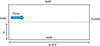 |
Fig. 1. Sketch of turbulent channel flow case. |
The coordinates and flow variables are normalized by the channel half-width δ, the friction velocity uτ, and the kinematic viscosity ν. For this case, the extended models for compressible flows, basic LienCubicKEBase and SugaCubicKE turbulence models are compared with DNS data [36] as well as with the analytical calculation of [37] of the dimensionless velocity and the turbulent viscosity profile (see in Figs. 2 and 3).
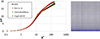 |
Fig. 2. Evolution of the dimensionless velocity profile. |
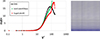 |
Fig. 3. Evolution of dimensionless turbulent viscosity profile. |
In the region y+ ≈ 10–100 (log-layer), both models closely match the DNS data for the dimensionless velocity. Minor deviations appear at higher y+ values, where both developed models slightly overestimate the DNS values. The profile of the dimensionless turbulent kinematic viscosity also agrees well with DNS data in the viscous sublayer. In the outer region (y+ > 80), the LienCubicKEBase model tends to overestimate the turbulent viscosity compared to the DNS. In contrast, the SugaCubicKE model shows better agreement with the DNS trend, although it exhibits a small peak that slightly exceeds the DNS values.
3.2. Rayleigh–Bénard convection case
The RBC case is a simple configuration for studying heat transfer via natural convection. It is provided by a limitless fluid layer enclosed by two fixed, horizontal, isothermal walls. The upper one is cooled, while the lower one is heated. The physical problem is characterized by the Rayleigh (Ra) and Prandtl number (Pr):
 (22)
(22)
 (23)
(23)
 |
Fig. 4. Computational domain for the RBC case. |
List of the RBC test cases.
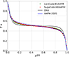 |
Fig. 5. Profiles of normalised temperature for RBC-I. |
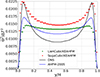 |
Fig. 6. Profiles of normalised temperature variance for RBC-I. |
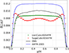 |
Fig. 7. Profile of normalised turbulent heat flux for RBC-I. |
where, ΔT is wall temperature difference, D is the distance between two horizontal walls, α is the thermal diffusivity, and Gr is the Grashof number. The RBC calculations are performed on a slender geometry with a 1:8 aspect ratio, assuming constant fluid properties using Boussinesq model. Figure 4 illustrates the computational domain of the RBC case. The 2D mesh consists of 3240 hexahedral cells (82 × 41) in total. Mesh analysis was performed with different mesh sizes: 40 × 20, 82 × 41 and 164 × 82 elements. The variation in the temperature field was very low. Therefore, the presented results shall be considered as mesh independent. Two vertical walls are treated as periodic boundaries in the horizontal direction, while the lower and upper walls are defined with no-slip conditions and maintained at constant wall temperatures, where (Th − Tc)≥1.
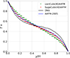 |
Fig. 8. Profiles of normalised temperature for RBC-II. |
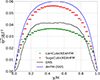 |
Fig. 9. Profiles of normalised temperature variance for RBC-II. |
In this study, the LienCubicKEAHFM and SugaCubicKEAHFM turbulence models are compared with DNS data and the solution from [9], referred here as AHFM-2005. The selected test cases are summarised in Table 4. For all the cases, the plot of T+ profile represents a normalised mean temperature defined as T + =(T−Tmin)/(Tmax−Tmin), the temperature variance is expressed as normalised temperature variance  , and the normalised turbulent heat flux is defined as
  . The channel height is represented in terms of the non-dimensional, wall-normal coordinate y/H. For the comparison of heat transfer, the Nusselt number (Nu) is derived using the following equation, where hc is the heat transfer coefficient and L is the characteristic length:
 (24)
(24)
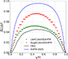 |
Fig. 10. Profile of normalised turbulent heat flux for RBC-II. |
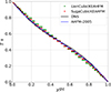 |
Fig. 11. Profile of normalised temperature for RBC-III. |
The simulation case RBC-I is characterised by Pr = 0.7 and Ra = 6.3 × 10⁵. The normalised mean temperature T+ profiles Figure 5 show good agreement between the turbulence models and DNS results. Both LienCubicKEAHFM and SugaCubicKEAHFM accurately capture the steep gradients near the thermal boundary layers and the linear behaviour in the bulk of the channel. Their performance compares well to DNS and is slightly better than AHFM-2005, although the DNS profile in the bulk is flatter than all numerical predictions. Figure 6 shows the thermal fluctuation behaviour represented by  . None of the models can quantitatively reproduce the DNS data, although AHFM-2005 and SugaCubicKEAHFM more or less follow the general profile trend. While SugaCubicKEAHFM is very close to the DNS data near the walls and captures the overall trend of the profile, it overestimates the temperature variance in the bulk by some 40%. The results with AHFM-2005 are better in the bulk region, while the peaks are underestimated significantly (approx. 35%). The performance of LienCubicKEAHFM is further away from the DNS data, in both, in the bulk and the near-wall regions and does not reproduce the peaks near the walls, which are present in the other three curves.
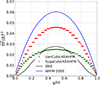 |
Fig. 12. Profiles of normalised temperature variance for RBC-III. |
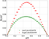 |
Fig. 13. Profile of normalised turbulent heat flux for RBC-III. |
The DNS data in of the normalised turbulent heat flux  (Fig. 7) shows a flat profile in the bulk and strong decay near the walls. LienCubicKEAHFM achieves the closest match from all simulations across the domain with a maximum deviation of 12% in the middle of the channel and with accurate prediction in the central and near-wall regions. SugaCubicKEAHFM predicts peaks in the near-wall regions and in the bulk, which are not in-line with the relatively flat DNS profile.
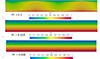 |
Fig. 14. T+ scalar field over the CFD domain calculated with LienCubicKEAHFM for Pr = 0.7 (top), Pr = 0.025 (middle) and Pr = 0.006 (bottom). |
The simulation case RBC-II is defined by Pr = 0.025 and Ra = 1 × 10⁵. In Figure 8, all models predict a somewhat flatter profile compared to the DNS one. Although the calculated trends are similar, AHFM-2005 and SugaCubicKEAHFM are closer to DNS. LienCubicKEAHFM predicts well in the central region, while slightly over- and underestimating the normalised temperature when moving towards bottom and top walls.
In the plot of  (Fig. 9) and
  (Fig. 10), LienCubicKEAHFM underestimates by 17% the variance and overestimates by 25% the turbulent heat flux, but still qualitatively accurately tracks the DNS profiles. SugaCubicKEAHFM and especially AHFM-2005 significantly overpredict the variance throughout the domain, with maximal deviations in the center of the channel. It was not easy to reach tight convergence in the RBC-II case with the developed models, specially LienCubicKEAHFM, which might explain the unexpected asymmetry in the profiles.
Figure 11 illustrates the profile of the normalised temperature for the RBC-III case with Pr = 0.006 and Ra = 2.4 × 10⁴. Here, all models including LienCubicKEAHFM and SugaCubicKEAHFM closely follow the DNS trend across the full height, accurately reproducing the nearly linear temperature gradient. In contrast, the normalized temperature variance throughout the domain is not reproduced by all models (Fig. 12). SugaCubicKEAHFM and AHFM-2005 models qualitatively represent the DNS profile shape, but significantly over predict the maximum value of the fluctuations. The LienCubicKEAHFM prediction of the temperature variance in the centre of the geometry is close to the DNS value, but unfortunately, the shape of the profile is flatter, and thus, differs from the reference one. Figure 13 presents the normalised turbulent heat flux, calculated with LienCubicKEAHFM and SugaCubicKEAHFM, DNS and AHFM-2005 were not available to compare with. The comparison of the two profiles is similar to the ones in RBC-I and RBC-II cases.
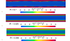 |
Fig. 15. Gradient of temperature field over the CFD domain calculated with LienCubicKEAHFM for Pr = 0.7 (top), Pr = 0.025 (middle) and Pr = 0.006 (bottom). |
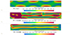 |
Fig. 16. Mean velocity distribution over the CFD domain calculated with LienCubicKEAHFM for Pr = 0.7 (top), Pr = 0.025 (middle) and Pr = 0.006 (bottom). |
Figure 14 presents the T+ field distribution, calculated with the LienCubicKEAHFM turbulence model for the three RBC cases. This figure is nearly identical to the one with the SugaCubicKEAHFM results (not shown here). In the case of RBC-I (Pr = 0.7), thermal plumes clearly rise and fall, which is typical for convection-dominated flows, where thermal diffusivity and momentum diffusivity are comparable (indication of strong convective mixing). For this case, the calculated Nusselt number is 6.7, which deviates by approximately 12% from the empirical solution in the literature [15]: Niemela – 7.53 (Nu = 0.124Ra0.309), Grossmann – 7.68 (Nu = 0.1Ra1/4 + 0.05Ra1/3). These correlations are valid for Prandtl number 0.7 and Rayleigh number between 106 ≤ Ra ≤ 1017.
As the Prandtl number decreases, the thermal boundary layer gets thicker. The Rayleigh number is also insufficient to drive strong convection, which results in isothermal layers that are mostly horizontal, indicating the dominance of the conduction with stratified temperature gradient (also visible in Fig. 15). This behaviour closely follows the DNS profile seen in Figure 11. The calculated Nusselt number for RBC-II and RBC-III are 1.9 and 1.19, which are lower than the result of the empirical solution of Rossby [38] – 2.83 (Nu = 0.147Ra0.257, Pr = 0.025, 103 ≤ Ra ≤ 5 × 10⁵), Kek [38] – 1.45 (Nu = 0.117Ra0.25, Pr = 0.006, 4 × 10⁴ ≤ Ra ≤ 2.5 × 10⁵). The possible reason for the lower Nu in our calculation might be the choice of AHFM model coefficients and parameters.
Figure 16 presents the velocity fields for RBC cases and illustrate how the flow structure changes with varying Ra and Pr numbers. In RBC-I (Ra = 6.3 × 10⁵, Pr = 0.7), the velocity distribution shows strong, coherent convection rolls, with smoothly varying regions of higher velocity concentrated near the centers of the convection cells (i.e. Fig. 14, RBC-I case). Because momentum and thermal diffusion occur on similar time scales at moderate Pr, the flow organizes into stable large-scale circulation patterns with velocity magnitudes on the order of 10−1. In RBC-II (Ra = 1 × 10⁵, Pr = 0.025), the dramatic drop in Prandtl number produces a very different behaviour. Thermal diffusion becomes dominant, weakening buoyancy-driven motion and generating thin, wavy, and irregular velocity structures (transitional or chaotic) rather than well-formed rolls. Velocities also decrease significantly, in the order of 10−5 to 10−4. RBC-III (Ra = 2.4 × 10⁴, Pr = 0.006) shows an even more diffusive (like laminar flow) and weakly convective regime, where both the lower Pr and lower Ra reduce flow intensity. The velocity field becomes smoother and more horizontally stretched, with minimal evidence of convection cells (smeared out), indicating a regime approaching conduction-dominated behaviour. Overall, the comparison highlights how decreasing Pr reduces the coherence of convection structures and how decreasing Ra further suppresses convective motion, resulting in progressively weaker and more diffused velocity fields across the three cases. The presented velocity distribution may vary depending on the selection of the governing parameters, see Table 3.
4. Conclusion and outlook
The commonly used eddy diffusivity approach has well-known limitations, which become particularly evident in advanced nuclear reactor applications that rely on liquid metal coolants such as sodium- and lead-cooled fast reactors. Deficiencies occur primarily in representation of natural and mixed convection regimes, being of particular importance in transient and accident conditions. The previously developed AHFM model at GRS was extended for compressible and incompressible flows within the framework of non-linear (cubic) turbulence models. The new developments were implemented in the HZDR’s NUSAR-RCS code, which is based on OpenFOAM.
It was shown that the predictions with the new models generally provide improved results compared to the ones, reported in the literature (AHFM-2005), but this is not always true for all investigated quantities. Deviations from DNS data in the shape and the magnitude of the evaluated profiles prove that further investigations are necessary. These shall aim at clarification of their origin, and further focus shall be put in the analysis of the different predictions of both implemented cubic k − ε turbulence models. Based on the discussed results, it is not easy to draw a final conclusion regarding the superiority of one of these models. Craft [40] proposed further correction in Suga’s model, which is currently under investigation at GRS. The analysis of the results may shed more light on the origin of deviations presented here.
The presented results are based on small scale academic test cases. In real life reactors, the geometries are very complex and the possible flow regimes, for example in normal and off-normal operational conditions, are quite different. Further, these regimes are not always steady and the transition between them further complicates the analysis of liquid metal flow and heat transfer phenomena. Therefore, these turbulence models must be further analysed and validated for reactor relevant conditions, before these can be applied for reactor safety analysis.
Funding
This work was funded by the German Federal Ministry for the Environment, Climate Action, Nature Conservation and Nuclear Safety within the UMRS 1607 project.
Conflicts of interest
The authors declare that they have no competing interests to report.
Data availability statement
The full description of performed work will be made publicly available within a report on the GRS website: https://www.grs.de/.
Author contribution statement
Conceptualization, Data curation, Formal analysis, Funding acquisition, Investigation, Methodology, Project administration, Resources, Supervision, Validation, Verification, Visualization, Writing – original draft, Writing – review & editing: – H. Mistry, J. Herb, A. Papukchiev.
Acknowledgments
This work was supported by the German Federal Ministry for the Environment, Climate Action, Nature Conservation and Nuclear Safety. The authors also acknowledge the kind support of HZDR in the implementation of the turbulence models in the NUSAR-RCS code.
Glossary
Glossary
AHFM: (Algebraic Heat Flux Model)
CFD: (Computational Fluid Dynamics)
DNS: (Direct Numerical Simulation)
GRS: (Gesellschaft f
HZDR: (Helmholtz-Zentrum Dresden-Rossendorf e.V.)
LFR: (Lead Fast Reactor)
LMFRs: (Liquid Metal Fast Reactors)
NLEVM: (Non-Linear Eddy Viscosity Model)
NUSAR-RCS: (Nuclear Safety Repository for OpenFOAM Foundation Software for Reactor Cooling System)
OECD/NEA: (Organisation for Economic Cooperation and Development (OECD)/Nuclear Energy Agency)
PWR: (Pressurized Water nuclear Reactor)
RANS: (Reynolds-Averaged Navier-Stokes equations)
RAS: (Reynolds Averaged Simulation)
RBC: (Rayleigh–B
SESAME: (Simulations and Experiments for the Safety Assessment of MEtal cooled rea-tor)
SFR: (Sodium Fast Reactor)
SGDH: (Simple Gradient Diffusion Hypothesis)
SIMPLE: (Semi-Implicit Method for Pressure-Linked Equations)
THINS: (Thermal-hydraulics of Innovative Nuclear Systems)
Roman symbols
aij: (Reynolds stress anisotropy tensor, −)
αf: (Non-uniform volume fraction field, −)
αt: (Turbulent thermal diffusivity, m2/s)
Cp: (Heat capacity of fluid, J/kg⋅K)
E: (Calculates near-wall turbulence energy dissipation, m2/s3)
e: (Internal energy, kg ⋅ m2/s2)
Fi: (Body force per unit mass, m/s2)
f2: (Damping function, −)
G: (Production of turbulence, m2/s3)
Gr: (Grashof number, −)
gi: (Gravitational acceleration, m/s2)
H: (Distance between two horizontal walls, m)
h: (Enthalpy, kg ⋅ m2/s2)
hc: (Heat transfer coefficient, W/m2K)
K: (Specific kinetic energy, m2/s2)
k: (Turbulence kinetic energy, m2/s2)
L: (Characteristic length, m)
Nu: (Nusselt number, −)
Pt: (Production of temperature variance, K2/s)
p: (Pressure, Pa)
Pr: (Prandtl number, −)
Prt: (Turbulent Prandtl number, −)
q: (Heat flux vector, W/m2)
qi: (Internal Energy Source, W/m3)
R: (Time-scale ratio, τθ/τm)
Ra: (Rayleigh number, −)
Re: (Reynolds number, −)
Reτ: (Reynolds number based on friction velocity, −)
Rt: (Turbulent Reynolds number, −)
SfvModels: (Source term using fvModels, −)
 :
(Non-dimensional strain rate, −)
:
(Non-dimensional strain rate, −)
Sij: (Mean strain rate tensor, 1/s)
T: (Temperature, K)
T+: (Normalized mean temperature, −)
T0: (Reference temperature, K)
t: (Time, s)
Ui: (Velocity component, m/s)
 :
(Turbulent momentum flux, m2/s2)
:
(Turbulent momentum flux, m2/s2)
x, y, z: (Direction, m)
y: (Wall normal distance, m)
y/H: (Non-dimensional wall-normal coordinate, −)
y*: (Dimensionless distance from the wall, −)
Yc: (Yap length scale correction m2/s4)
Greek symbols
α: (Thermal diffusivity, m2/s)
β: (Thermal expansion coefficient, 1/K)
δij: (Kronecker delta, −)
ΔT: (Temperature difference, K)
ε: (Turbulent kinetic energy dissipation rate, m2/s3)
εθ: (Dissipation rate of temperature variance, K2/s)
η: (Suga turbulence model coefficient, −)
 :
(Temperature variance, K2)
:
(Temperature variance, K2)
 :
(Normalized temperature variance, −)
:
(Normalized temperature variance, −)
 :
(Turbulent heat flux, K⋅m/s)
:
(Turbulent heat flux, K⋅m/s)
 :
(Normalised turbulent heat flux, m/s)
:
(Normalised turbulent heat flux, m/s)
κ: (Thermal conductivity of fluid, W/m⋅K)
κc: (Constant coefficient of wall function calculation, 0.41)
μ: (Dynamic viscosity, Pa⋅s)
μt: (Turbulent dynamic viscosity, Pa⋅s)
ν: (Kinematic turbulent viscosity, m2/s)
νt: (Eddy viscosity, m2/s)
ρ: (Fluid density, kg/m3)
τm: (Mechanical time-scale, s)
τθ: (Thermal time-scale, s)
 :
(Non-dimensional vorticity rate, −)
:
(Non-dimensional vorticity rate, −)
Ωij: (Mean vorticity rate tensor, 1/s)
References
- Generation IV International Forum (GIF): Technology Roadmap Update for Generation IV Nuclear Energy Systems, (2014), https://www.gen-4.org/gif/upload/docs/application/pdf/2014-03/gif-tru2014.pdf Accessed 24 January 2020 [Google Scholar]
- S.J. Zinkle, G.S. Was, Materials challenges in nuclear energy, Acta Materialia (2013), https://doi.org/10.1016/j.actamat.2012.11.004 [Google Scholar]
- M. Xing, J. Fan, F. Shen, D. Lu, L. Li, H. Yu, J. Fan, Comparative analysis on the characteristics of liquid lead and lead-bismuth eutectic as coolants for fast reactors, Energies 18, 596 (2025), https://doi.org/10.3390/en18030596 [Google Scholar]
- OECD/NEA: Benchmark Analyses of Sodium Natural Convection in the Upper Plenum of the Monju Reactor Vessel, Final Report of a Coordinated Research Project 2008-2012, IAEA-TECDOC-1754, IAEA, https://www.osti.gov/etdeweb/servlets/purl/22300443 (2014) [Google Scholar]
- A. Papukchiev, F. Roelofs, A. Shams, G. Lecrivain, W. Ambrosini, Development and application of computational fluid dynamics approaches within the European project THINS for the simulation of next generation nuclear power systems, Nucl. Eng. Design 290, 13 (2015), https://doi.org/10.1016/j.nucengdes.2014.12.003 [Google Scholar]
- D. Wilcox, Turbulence Modeling for CFD, 3rd edn. (DCW Industries, 2006) [Google Scholar]
- M. Escudier. Introduction to Engineering Fluid Mechanics, 1st edn. (Oxford University Press, 2017) [Google Scholar]
- A. de Santis, A. Shams, Application of an algebraic turbulent heat flux model to a backward facing step flow at low Prandtl number, Ann. Nucl. Energy (Oxford) 117, 32 (2018) https://doi.org/10.1016/j.anucene.2018.03.016 [Google Scholar]
- A. Shams, F. Roelofs, E. Baglietto, S. Lardeau, S. Kenjeres, Assessment and calibration of an algebraic turbulent heat flux model for low-Prandtl fluids, Int. J. Heat and Mass Transfer 79, 589 (2014), https://doi.org/10.1016/j.ijheatmasstransfer. 2014.08.018 [Google Scholar]
- G. Groetzbach, Turbulence modelling issues in ADS thermal and hydraulic analyses, IAEA Technical Meeting on Theoretical and Experimental Studies of Heavy Liquid Met-al Thermal Hydraulics, Karlsruhe, Germany, Oct. 28-31 (2003). IAEA-TECDOC-1520.IAEA Wien, Oct. 2006, pp. 9–32 (2003) [Google Scholar]
- A. Papukchiev, Experimental validation of ANSYS CFX for transient flows with heat transfer in a tubular heat exchanger, J. Nucl. Eng. Radiat. Sci. 6, 021104 (2020), https://doi.org/10.1115/1.4045074 [Google Scholar]
- W. Rodi, Turbulence Models and Their Application in Hydraulics: A State-of-the Art Re-View, 3rd edn. (IAHR Monographs, A.A. Balkema, Rotterdam, Netherlands, 1993) [Google Scholar]
- M. Jischa, H.B. Rieke, About the prediction of turbulent Prandtl and Schmidt numbers from modeled transport equations, Int. J. Heat & Mass Transf. 22, 1547 (1979), https://doi.org/10.1016/0017-9310(79)90134-0 [Google Scholar]
- W.M. Kays, Turbulent Prandtl number. Where are we? J. Heat Transf. 116, 284 (1994) [Google Scholar]
- S. Kenjereš, K. Hanjalić, Convective rolls and heat transfer in finite-length Rayleigh-Bénard convection: A two-dimensional numerical study, Phys. Rev. E 62, 7987 (2000), https://doi.org/10.1103/PhysRevE. 62.7987 [Google Scholar]
- R. So, L.H. Jin, T.B. Gatski, An explicit algebraic Reynolds stress and heat flux model for incompressible turbulence: Part II Buoyant flow, Theor. Comput. Fluid Dyn. 17, 377 (2004), https://doi.org/10.1007/ s00162-004-0123-7 [Google Scholar]
- S. Kenjereš, S.B. Gunarjo, K. Hanjalić, Contribution to elliptic relaxation modelling of turbulent natural and mixed convection, Int. J. Heat Fluid Flow 26, 569 (2005), https://doi.org/10.1016/j.ijheatfluidflow. 2005.03.007 [Google Scholar]
- A. Shams, F. Roelofs, E. Baglietto, S. Lardeau, S. Kenjeres, Assessment of an algebraic heat flux model for the applications of innovative reactors, 15th edn., in The 15th International Topical Meeting on Nuclear Reactor Thermalhydraulics, NURETH-15-276, Pisa, Italy, 2013 [Google Scholar]
- V. Habiyaremye, A. Mathur, F. Roelofs, Modeling of forced convection in low-Prandtl-number fluids using a novel local algebraic heat flux model, Nucl. Sci. Eng. 199, 1643 (2024), https://doi.org/10.1080/00295639.2024.2400765 [Google Scholar]
- S. Manservisi, F. Menghini, A CFD four parameter heat transfer turbulence model for engineering applications in heavy liquid metals, Int. J. Heat & Mass Transf. 69, 312 (2014) [Google Scholar]
- A. Seubert, M. Behler, J. Bousquet, R. Henry, J. Herb, G. Lerchl, P. Sarkadi, Weiter-entwicklung der Rechenmethoden zur Sicherheitsbewertung innovativer Reaktorkonzepte mit Perspektive P&T, GRS-Bericht, GRS-553, Gesellschaft für Anlagen- und Reaktorsicherheit (GRS) gGmbH, Köln, Garching b. München, Berlin, Braunschweig, 2019 [Google Scholar]
- F.S. Lien, W.L. Chen, M.A. Leschziner, Low-reynolds-number eddy-viscosity modelling based on non-linear stress-strain/vorticity relations, in Engineering Turbulence Modelling and Experiments Elsevier Series in Thermal and Fluid Sciences, edited by W. Rodi (Elsevier, Oxford, 1996), pp. 91-100 [Google Scholar]
- D. Apsley, Turbulence Modelling in STREAM (2002), https://personalpages.manchester.ac.uk/staff/ david.d.apsley/turbmod.pdf [Google Scholar]
- OpenFOAM Foundation: Release Notes of OpenFOAM 7 (2019), https://openfoam.org/release/7/ [Google Scholar]
- OpenFOAM Foundation: Release Notes of OpenFOAM 12 (2024), https://openfoam.org/release/12/ [Google Scholar]
- HZDR: NUSAR-RCS, Project number 1501658, HZDR 2025, https://www.hzdr.de/db/Cms?p0id=65162&pid= 121 Accessed 2025] [Google Scholar]
- Roelofs, F. (ed.), Thermal Hydraulics Aspects of Liquid Metal Cooled Nuclear Reactors (Woodhead Publishing, 2019) [Google Scholar]
- Thermal-hydraulics of Innovative Nuclear Systems (THINS), ID 249337, (2015), https://cordis.europa.eu/project/id/249337/reporting [Accessed 2025] [Google Scholar]
- M. Tarantino, F. Roelofs, A. Shams, A. Batta, V. Moreau, I. Di Piazza, A. Gerschenfeld, P. Planquart, SESAME project: Advancements in liquid metal thermal hydraulics experiments and simulations, EPJ Nuclear Sci. Technol. 6, 18 (2020), https://doi.org/10.1051/epjn/2019046 [Google Scholar]
- S. Kenjereš, Numerical modelling of complex buoyancy-driven flows. Ph.D. thesis, Delft University of Technology, 1998 [Google Scholar]
- K. Suga, Development and application of a non-linear eddy-viscosity model sensitized to stress and strain invariants. Ph.D. thesis, Faculty of Technology, University of Manchester, 1995 [Google Scholar]
- T.J. Craft, B.E. Launder, K. Suga, Development and application of a cubic eddy-viscosity model of turbulence, Int. J. Heat Fluid Flow, 17, 108 (1996), https://doi.org/10.1016/0142-727X (95)00079-6 [Google Scholar]
- C.R. Yap, Turbulent heat and momentum transfer in recirculating and impinging flow. Ph.D. thesis, Faculty of Technology, University of Manchester, 1987 [Google Scholar]
- B.E. Launder, B.I. Sharma, Application of the energy-dissipation model of turbulence to the calculation of flow near a spinning disc, Lett. Heat Mass Trans. 1(2), 131 (1974), https://doi.org/10.1016/0094-4548(74) 90150-7 [Google Scholar]
- Z. Wei, B. Ničeno, R. Puragliesi, E. Fogliatto, Assessment of turbulent heat flux models for URANS simulations of turbulent buoyant flows in ROCOM tests, Nucl. Eng. Technol. 54, 4359 (2022), https://doi.org/10.1016/j.net. 2022.07.009 [Google Scholar]
- H. Abe, R.A. Antonia, H. Kawamura, Correlation between small-scale velocity and scalar fluctuations in a turbulent channel flow, J. Fluid Mech. 627, 1 (2009) [Google Scholar]
- J. Kim, P. Moin, R. Moser, Turbulence statistics in fully developed channel flow at low Reynolds number, J. Fluid Mech. 177, 133 (1987) [CrossRef] [Google Scholar]
- M. Wörner, Direkte simulation turbulenter rayleigh-bénard-konvektion in flüssigem natrium, Kern-forschungszentrum Karlsruhe, kfk 5228, (1994) [Google Scholar]
- I.Otić, G. Grötzbach, M. Woerner, Analysis and modelling of the temperature variance equation in turbulent natural convection for low-Prandtl-number fluids, J. Fluid Mech. 525, 237 (2005) [Google Scholar]
- T.J. Craft, H. Iacovides, J.H. Yoon, Progress in the use of non-linear two-equation models in the computation of convective heat-transfer in impinging and separated flows, Flow, Turbul. Combust. 63, 59 (2000), https://doi.org/ 10.1023/A:1009973923473 [Google Scholar]
Cite this article as: Hemish Mistry, Joachim Herb, Angel Papukchiev, Extension of the turbulent heat flux modelling in OpenFOAM for improved simulation of liquid metal flows, EPJ Nuclear Sci. Technol. 12, 8 (2026), https://doi.org/10.1051/epjn/2025079
Appendix
A. Turbulence model: LienCubicKEBase
Class:
Foam::RASModels::LienCubicKEBase
Header location:
$FOAM_SRC/MomentumTransportModels/momentumTransportModels/RAS/LienCubicKEBase/
Purpose:
The LienCubicKEBase model is a reformulated extension of the LienCubicKE turbulence model, constructed to ensure consistent behaviour in both compressible and incompressible flows and implemented in OpenFOAM through density- and volume-fraction-weighted transport equations for k and ε.
Main Components:
-
Model coefficients: Defined in LienCubicKEBase.C and adjustable via RASProperties.
-
Turbulent viscosity calculation: Involves cubic terms of the strain-rate and vorticity tensors.
-
solve() routine: Handles sequential solution of k and ε equations each iteration.
-
Correct() loop: Updates turbulent viscosity and non-linear stress contributions.
Users call:
 In constant/momentumTransport
  RAS
  {
    RASModel    LienCubicKEBase;
    turbulence  on;
  }
B. fvModels: energyAHFM
Class:
Foam::fv::energyAHFM
Header location:
$FOAM_SRC/fvModels/derived/energyAHFM/
Purpose:
The Algebraic Heat Flux Model (AHFM) provides a source term for the energy or temperature equation in compressible and incompressible flow simulations. It is specifically intended to operate consistently with the LienCubicKEAHFM and SugaCubicKEAHFM momentum transport models.
Users call:
 In constant/fvModels
  energyAHFM1
  {
    type    energyAHFM;
    libs    ("libaddonfvModels.so");
  }
C. fvModels: incompressible Buoyancy Force
Class:
Foam::fv::incompressibleBuoyancyForce
Header location:
$FOAM_SRC/fvModels/derived/incompressibleBuoyancyForce/
Purpose:
Evaluates the buoyancy contribution according to the Boussinesq approximation, expressed as (1 − β(T − T0)) and incorporates it into the incompressible momentum equation for the specified velocity field. Intended to work with incompressible turbulence models.
Users call:
 In constant/fvModels
 incompressibleBuoyancyForce1
 {
  type    incompressibleBuoyancyForce;
  libs    ("libaddonfvModels.so");
  U       U; // Name of the velocity field
  T       T; // Name of the temperature field
  beta    beta; // Name of the thermal expansion field
 }
All Tables
All Figures
|
Fig. 1. Sketch of turbulent channel flow case. |
| In the text | |
|
Fig. 2. Evolution of the dimensionless velocity profile. |
| In the text | |
|
Fig. 3. Evolution of dimensionless turbulent viscosity profile. |
| In the text | |
|
Fig. 4. Computational domain for the RBC case. |
| In the text | |
|
Fig. 5. Profiles of normalised temperature for RBC-I. |
| In the text | |
|
Fig. 6. Profiles of normalised temperature variance for RBC-I. |
| In the text | |
|
Fig. 7. Profile of normalised turbulent heat flux for RBC-I. |
| In the text | |
|
Fig. 8. Profiles of normalised temperature for RBC-II. |
| In the text | |
|
Fig. 9. Profiles of normalised temperature variance for RBC-II. |
| In the text | |
|
Fig. 10. Profile of normalised turbulent heat flux for RBC-II. |
| In the text | |
|
Fig. 11. Profile of normalised temperature for RBC-III. |
| In the text | |
|
Fig. 12. Profiles of normalised temperature variance for RBC-III. |
| In the text | |
|
Fig. 13. Profile of normalised turbulent heat flux for RBC-III. |
| In the text | |
|
Fig. 14. T+ scalar field over the CFD domain calculated with LienCubicKEAHFM for Pr = 0.7 (top), Pr = 0.025 (middle) and Pr = 0.006 (bottom). |
| In the text | |
|
Fig. 15. Gradient of temperature field over the CFD domain calculated with LienCubicKEAHFM for Pr = 0.7 (top), Pr = 0.025 (middle) and Pr = 0.006 (bottom). |
| In the text | |
|
Fig. 16. Mean velocity distribution over the CFD domain calculated with LienCubicKEAHFM for Pr = 0.7 (top), Pr = 0.025 (middle) and Pr = 0.006 (bottom). |
| In the text | |
Current usage metrics show cumulative count of Article Views (full-text article views including HTML views, PDF and ePub downloads, according to the available data) and Abstracts Views on Vision4Press platform.
Data correspond to usage on the plateform after 2015. The current usage metrics is available 48-96 hours after online publication and is updated daily on week days.
Initial download of the metrics may take a while.