| Issue |
EPJ Nuclear Sci. Technol.
Volume 11, 2025
Status and advances of Monte Carlo codes for particle transport simulation
|
|
|---|---|---|
| Article Number | 11 | |
| Number of page(s) | 11 | |
| DOI | https://doi.org/10.1051/epjn/2025008 | |
| Published online | 24 April 2025 | |
https://doi.org/10.1051/epjn/2025008
Regular Article
ARCHER-a Monte Carlo code for multi-particle radiotherapy through GPU-accelerated simulation and DL-based denoising
1
School of Nuclear Science and Technology, University of Science and Technology of China Hefei 230026 C.R. China
2
Anhui Wisdom Technology Company Limited Hefei 230000 C.R. China
3
Shanghai Proton and Heavy Ion Center Shanghai 201215 C.R. China
* e-mail: This email address is being protected from spambots. You need JavaScript enabled to view it.
Received:
21
June
2024
Received in final form:
13
January
2025
Accepted:
17
March
2025
Published online: 24 April 2025
Abstract
The ARCHER project was initiated about 14 years ago to explore the use of emerging GPU technologies for fast Monte Carlo (MC) calculations. This paper presents the latest work to integrate the newly developed deep conventional neural network (dCNN) based MC denoising method with GPU-based MC multi-particle radiation transport simulation method to demonstrate a real-time dose computing capability for clinically realistic radiotherapy examples. The computing process involves GPU-based dose calculations that is followed by dCNN-based denoising. The dCNN-based dose denoiser is designed and employed to reduce the statistical uncertainty in dose distributions in patient anatomy defined by 3D computed tomography (CT) images. The training data include a range of dose distributions covering low-count/high-noise (DoseLCHN) and high-count/low-noise (DoseHCLN). The extremely large DoseLCHN and DoseHCLN dataset was generated from ARCHER. The DoseLCHN dataset is input into the trained model to output a predicted DoseHCLN dataset. For the evaluation, the DoseHCLN dataset produced by ARCHER is considered to be the ground truth. Experimental results show that the dose distributions generated from newly proposed method agreed consistently with the DoseHCLN produced from ARCHER. For hundreds of patient radiation treatment cases involving photons and protons, the average running time for one patient (GPU-based dose simulation followed by dCNN-based denoising) is about 200 ms. These preliminary results have demonstrated the feasibility of real-time Monte Carlo dose computing using an integrated dCNN-based denoising and GPU-based dose calculational approach. On-going studies involving more radiation types and clinical procedures are expected to facilitate the use of real-time MC dose planning and verification in the clinical workflow.
© Y. Chang et al., Published by EDP Sciences, 2025
 This is an Open Access article distributed under the terms of the Creative Commons Attribution License (https://creativecommons.org/licenses/by/4.0), which permits unrestricted use, distribution, and reproduction in any medium, provided the original work is properly cited.
1. Introduction
ARCHER (Accelerated Radiation-transport Computations in Heterogeneous EnviRonments) is a Monte Carlo radiation transport code that has been under development since 2010. Driven by needs for energy-efficiency in peta- and exa-scale supercomputers, heterogeneous system designs involving hardware accelerators such as NVIDIA graphics processing units (GPUs) emerged. Intel Xeon Phi Many-Core-Coprocessors (MICs) –which were no longer supported by INTEL –were once a strong competitor to GPUs. As a GPU-based Monte Carlo radiation transport testbed ARCHER was designed to have CPU, GPU and MIC versions at Rensselaer Polytechnic Institute (Troy, New York, USA) to show the feasibility under emerging heterogeneous computing environments [1–3]. It was clear to us 14 years ago that none of the existing general-purpose MC radiation transport codes used in nuclear engineering [4–10] were designed to take advantage of the computation capabilities afforded by these heterogeneous computer architectures which many believed would soon play vital roles. One challenge had to do with the prohibitive amount of re-programming time required before an existing MC code may be implemented for GPU/CUDA, or similar architectures. The uncertainty surrounding the final hardware/software specifications in future supercomputers had kept many end-users from playing an active role in the emerging field of “GPU-based” MC development [2]. We are one of the several groups that have managed to make breakthroughs in designing new, GPU-based MC codes [1–3, 11–14].
A lot of attempts have been made to accelerate MC methods. By simplifying physics models, many have developed fast MC algorithms that are effective for specific applications but difficult to adapt for other situations (e.g., [15]). GPU-based MC codes have emerged to boost extensive thread-level parallelism and high energy efficiency. Since MC algorithms are compute-intensive but parallelizable, they can be offloaded to GPU and be concurrently executed by thousands of threads [16]. In the process of clinical radiotherapy, dose calculation needs to be implemented during planning and dose validation. If the speed of dose calculation is very slow, it will occupy and waste equipment and personnel resources, so calculating for a few hours is not enough to meet clinical requirements. The GPU-based MC code, ARCHER, can achieve simulation times in less than one minute using the latest GPU devices (e.g., [17–19]), including the time for cross section initialization, transmission in multi-leaf collimator (MCL) and transmission in human body. The level of computing efficiency meets the clinical workflow, clinical workers can quickly see the results and continue clinical work. However, in certain areas of modern radiotherapy, such as offline/online “adaptive radiotherapy (ART)” where tomographic images are used to adjust treatment dose margins for every fraction of the treatment, MC dose calculations should ideally be completed in sub-second [20, 21], which can reduce changes in the patient's anatomical structure and improve the accuracy of dose delivery.
Can we further decrease the time of MC simulation? The more particles simulated by Monte Carlo, the lower the statistical uncertainty of each voxel (lower error), and the more accurate the calculated dose distribution, The concept of “Monte Carlo denoising” using deep learning (DL) technologies was proposed in 2019 [22] and the interest from the research community has since been rising [23–28]. Together, these studies have demonstrated the feasibility of using convolutional neural network (CNN)-based deep learning (DL) techniques to reduce the noise in Monte Carlo simulations with promising results. For instance, Peng et al. [22] and Bai et al. [25] designed a 2D convolutional encoder-decoder neural network and a lightweight DL-based CNN for fast MC dose denoising in intensity-modulated radiation therapy involving photons. Zhang G et al. [27] and Zhang X et al. [28] have successfully denoised the MC dose maps for proton and Carbon ion therapy with ResNet networks and GhostUNet networks, respectively. There is still a need to integrate GPU-based first-principal MC simulations with DL-based denoising methods leading eventually to what we call “real-time” (sub-seconds) MC simulations.
In this study, we combine GPU-accelerated Monte Carlo simulation method with DL-based denoising method for radiotherapy dose calculations. First, ARCHER, a GPU-based MC software previously developed by our group, is used to generate the training dataset, including low-count/high-noise dose distribution (DoseLCHN) and high-count/low-noise dose distribution (DoseHCLN). Then, the dCNN-based dose denoiser is designed and employed to reduce the statistical uncertainty in dose distributions. Clinical patient data are collected for this study to validate the accuracy and efficiency of proposed methods.
2. Methods and materials
We introduce ARCHER from two aspects, GPU-based Monte Carlo method and AI-based denoising method. For GPU-based Monte Carlo method, ARCHER has realized multi-particle calculation algorithms including photons, electrons, protons and heavy ions (work on neutrons is in progress). Results for DL-based denoising method are reported here for photon radiotherapy and proton radiotherapy.
2.1. GPU-based Monte Carlo simulation methods
2.1.1. Photons
The photon-electron coupled Monte Carlo dose calculation includes two major parts: host code that runs on the CPU and the device code (also called kernel) that runs on the GPU (shown in Fig. 1). The general code structure follows a typical CUDA execution pattern: first the host code is executed to read in data and transfer data from host memory to device memory. Then the kernel code is called by the host code and it is executed on the GPU in parallel with multiple threads.
 |
Fig. 1. Flowchart of ARCHER code involving CPU-GPU heterogeneous structure. RNG means random number generator, PSF means phase space file. The left panel describes the work for CPU which is the host and the right panel describes the work for GPU which is the device. Device cannot interact with outer world directly and can only send/receive data to/from host. Host and device communicate via PCI-E bus. Host first reads data and sends them to device; after simulation, device sends results back to host. Pseudorandom number (PRN) kernel is used to initiate the PRN streams. Transport kernel handles the MC simulation of particles. Batch simulation is employed. After all batches are done, the host synchronizes all thread on the device and processes and outputs results. |
For photon transport, the main physics models implemented in ARCHER were similar to production MC codes, we considered photoelectric effect, Compton scattering and pair production. Rayleigh scattering is disregarded in this study because it has negligible impact on dose distribution for photon energy range used for radiotherapy. Compton scattering is sampled according to the Klein-Nishina cross section, assuming electrons are free and at rest before scattering. The photoelectric effect is modeled by ignoring electron shell structure and binding energy. A secondary electron is produced isotropically with the same energy of the incident photon. For pair production, the electron and positron are assumed to split the incident photon energy using a uniformly distributed random number. More detailed information is described in our previous studies [1, 17, 18].
2.1.2. Protons
ARCHER simulates proton transport in voxelized geometry from computed tomography (CT) scans with kinetic energy up to 300 MeV. The Hounsfield Unit (HU) of each voxel is converted into density and elemental composition. There are 13 elements and 24 materials predefined. Protons interact with media through various electromagnetic and nuclear interactions. Due to the large number of elastic Coulomb interactions, the analog event-by-event simulation is unfeasible. Therefore, the so-called class-II condensed history method with a continuously slowing down approximation is employed. Each proton is tracked step-by-step until its energy drops below 0.5 MeV or exits the boundary of the phantom. More detailed information is described in our previous study [19].
2.1.3. Neutrons
According to the report of IAEA [29], the primary dose components and sources in the BNCT process are outlined in Table 1. Therefore, for neutron transport in BNCT scenarios, we must consider elastic scattering, inelastic scattering, and capture reactions involving neutrons and various elements. For thermal neutrons with energies below 4 eV, the S(α, β) model is employed to simulate thermal scattering. Our program utilizes continuous energy, with nuclear data derived from the latest ENDF VIII.0 nuclear database [30].
Four dose components of BNCT.
During BNCT, secondary particles primarily consist of heavy charged particles and photons. These heavy charged particles in BNCT have limited ranges in the human body. For instance, the range of Li-7 and α particles in the human body is comparable to the diameter of a cell (∼10 μm). Secondary protons and other heavy charged particles (such as C-14), possess kinetic energies of at most a few MeV, corresponding to ranges of only a few millimeters in the human body. Consequently, it can be assumed that heavy charged particles deposit their energy locally, and the main focus should be on the transport of secondary photons.
Our program was initially developed as a pure CPU version using C++ and then rewritten with CUDA for parallel computation on the GPU. Considering the initial development and maintenance needs, the current implementation of neutron transport simulation on the GPU uses the history-based algorithm. For GPU memory configuration, various local variables are allocated in registers to enable fast access. Shared memory is used to store the counting results of all threads within a block. Neutron cross-sections, thermal scattering S(α, β) data, and geometric parameters remain constant during the simulation and are shared by all threads, thus they are stored in constant memory. The generated secondary photons are stored in global memory and are simulated only after the completion of all primary neutron simulations.
2.1.4. Heavy ions
ARCHER performs simulations of helium ions (4He) transport with kinetic energy levels of up to 220 MeV/u, corresponding to a range of approximately 30 cm in water. 4He undergo a step-by-step transport process until their energy drops below 1 MeV/u or until they exit the phantom. The entire simulation is divided into three transport kernel functions: one for 4He, one for secondary deuterons, tritons, and 3He, and one for protons. We keep one particle heap memory in the 4He kernel function to store secondary particles that will be simulated in the next two kernel functions. For each secondary particle, the type, the kinetic energy, the location, and the direction are stored. When different threads attempt to write secondary particles to the heap memory, however, it can easily lead to issues of read-write conflicts. To mitigate this conflict, the memory is evenly distributed among multiple threads, with each thread being allowed to operate only on the heap memory allocated to it. To guarantee that each thread has enough allocated heap memory, the memory size must exceed the size of all secondary particles, which is an empirical value and set to twice the number of primary 4He. After the 4He kernel function, secondary particles are sorted and categorized by energy and type. Although this may take some additional time, it minimizes divergence in the next two kernel functions, thereby reducing the simulation time.
2.2. DL-based denoising
As illustrated in Figure 2, the dCNN-based dose denoiser was designed and employed to reduce the statistical uncertainty in dose distributions of 3D patient CT phantoms. The training included a range of data covering low-count and high-noise (DoseLCHN) and high-count and low-noise (DoseHCLN). As a unique feature of this study, an extremely large DoseLCHN and DoseHCLN dataset was generated from ARCHER–a GPU-based MC software previously developed by our group–for photon, proton radiotherapy cases. In the testing, the DoseLCHN dataset was input into the trained dCNN model to output a predicted high-count and low-noise DoseHCLN dataset. To evaluate the performance of proposed method, the DoseHCLN dataset produced by the well-validated ARCHER code was considered to be the ground truth.
 |
Fig. 2. Monte Carlo (MC) simulation denoising neural network flow chart. The definition of gamma test can be seen in reference [31]. |
The Monte Carlo Denoising Network (MCDNet), initially reported in our early work [22, 23], was designed for 2D data. In this study, we improved it to a 3D structure to better accommodate the training of 3D data. Figure 3 illustrates the network architecture of the 3D MCDNet. 3D MCDNet comprises an encoder and a decoder. The encoder includes five convolutional modules, each consisting of a 3 × 3 × 3 convolutional layer followed by a ReLU activation layer. In contrast, the decoder includes five deconvolution modules, each consisting of a convolutional layer and a deconvolution layer. Four black dashed arrows in the figure indicate four conveying paths, which copy and reuse early feature maps as inputs for subsequent layers with the same feature map size, preserving high-resolution features. Such a mechanism can reduce the search space of the network's output, facilitating faster convergence. The black solid lines represent residual skip connections that sums up the network's input and output features, enabling the network to infer the noise from the input image directly. Moreover, MCDNet is akin to the well-known U-Net, used for biomedical imaging segmentation, but it avoids the down-sampling operations that may lead to loss of detail. Such theoretical analysis ensures that MCDNet can achieve the reasonable performance.
 |
Fig. 3. The architecture of dose denoising network. |
3. Results
3.1. Results of GPU-based Monte Carlo dose calculations
Several general-purpose MC codes were used to validate the accuracy of GPU-based Monte Carlo algorithms in ARCHER. Figure 4 compares photon dose distributions by ARCHER and GEANT4 showing excellent agreement between the two codes [1, 17]. In similar ways, Figure 5 compares proton dose calculations by ARCHER and TOPAS [19], Figure 6 compares Boron Neutron Capture Therapy simulations by ARCHER and GEANT4 and, finally, Figure 7 compares Helium dose calculations by ARCHER and TOPAS. These extensive comparisons are necessary to verify the accuracy of radiological physics models in ARCHER for various particles.
 |
Fig. 4. Comparison of prostate treatment dose distributions showing excellent agreement. (a) ARCHER results. (b) GEANT4 results. The similarity of the contour lines from two MC codes is obvious showing the satisfactory accuracy in dose calculations by ARCHER. |
 |
Fig. 5. Dose comparison in water for proton dose calculation. (a) Integrated depth-dose profiles are shown. TOPAS simulations are indicated by solid red lines, ARCHER simulations as blue points, and the relative errors are plotted in green and gray dots. (b) Two lateral profiles for 100 MeV proton beam are shown. The legend “50 mm” represents the lateral profile obtained at the depth of 50 mm. (c) Lateral profiles for the 200 MeV proton beam are shown. |
 |
Fig. 6. Comparison of neutron flux and different dose component of Boron Neutron Capture Therapy in a phantom. (a) fast neutron dose, (b) boron dose, (c) photon dose. |
 |
Fig. 7. Dose comparison in water for Helium dose calculations. (A) Integrated depth-dose profiles are shown. ARCHER simulations are in solid red lines, TOPAS simulations are in blue points, and the relative errors are plotted in green, purple, and black dots for 100 MeV/u, 150 MeV/u, and 20 MeV/u respectively. (B) Three lateral profiles for 200 MeV 4He are shown. The legend “257 mm” represents the lateral profile obtained at the depth of 257 mm. |
3.2. Results of DL-based denoising
The work for DL-based denoising was performed using the following hardware:
-
CPU: AMD EPYC 7763
-
CPU cores: 64
-
CPU threads: 128
-
Memory: 512GB
-
GPU: NVIDIA RTX 3090
-
GPU memory: 24GB
Clinical photon radiotherapy data include 66 rectal cancer patients treated with intensity modulated radiotherapy (IMRT) and 66 cervical cancer patients treated with volumetric modulated arc therapy (VMAT). Proton radiotherapy data consist of 83 head and neck cancer patients and 83 pelvis patients treated on SIEMENS IONTRIS system. Each treatment site was divided into training, validation and testing datasets according to 4:1:1. The gamma pass rate (GPR, 2%/2 mm) and root mean squared error (RMSE) were calculated to evaluate the denoising method.
The results of photon radiotherapy are shown in Figure 8 and Table 2. The dose maps by simulating 1 × 10⁹ counts are regarded as the ground truth for comparison. As shown in Figure 8, the dose map generated by running 1 × 10⁶ photons contains much noise (due to statistical uncertainty), while the denoised dose map has clearly less noise in the dose distributions. As summarized in Table 2, the DL-based denoising method can improve the GPR (2%/2 mm) from 87.9% (by 1 × 10⁶ photons) to 98.2% (denoised) for rectal cancer patients, from 68.9% (1 × 10⁶ photons) to 93.4% (denoised) for cervical cancer patients. In terms of computational performance, the total time for 1 × 10⁹ photons is 26.6 s and 28 s for rectal and cervical patients, respectively, while the time for 1 × 10⁶ photons is 96 ms and 138 ms for rectal and cervical patients, respectively. Table 2 also indicates that the model prediction time (i.e., the time for the trained dCNN to perform the task of denoising) is 15 ms. That is to say, the total computing time to obtain a dose distribution equivalent to that produced from 1 × 10⁹ photons is reduced from 26.6 s and 28 s – for rectal and cervical patients, respectively – to 0.111 s (96 ms + 15 ms) and 0.151 s (138 ms + 15 ms) assuming comparable global dose accuracy.
 |
Fig. 8. Monte Carlo dose distributions having different simulated photon numbers for radiotherapy of rectal cancer and cervical cancer in terms of predicted and ground-truth data (standard deviation <1%). The numbers in parentheses are simulated numbers of photons. |
Summary of DL-based denoising for photon radiotherapy data.
The results of proton radiotherapy are summarized in Figure 9 and Table 3 showing somewhat similar characteristics as those of photon radiotherapy. The dose maps by simulating 1 × 10⁸ protons are regarded as the ground truth for comparison. In Table 3, the DL-based denoising method can improve the GPR (2%/2 mm) from 70.6% (by 1 × 10⁶ protons) to 96.2% (denoised) for head and neck cancer patients, from 82.5% (1 × 10⁶) to 94.4% (denoised) for pelvic cancer patients. In terms of the simulation time, the time for 1 × 10⁸ counts is 25 s and 28 s for head-and-neck patients and pelvic patients, respectively, the time for 1 × 10⁶ protons is 153 ms and 187 ms, respectively. The model prediction time is 15 ms. In a short summary, the total computing time to obtain a dose distribution equivalent to that produced from 1 × 10⁸ protons is reduced from 25 s and 28 s – for head-and-neck and cervical patients, respectively – to 0.168 s (153 ms + 15 ms) and 0.202 s (187 ms + 15 ms) assuming comparable global dose accuracy.
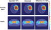 |
Fig. 9. Monte Carlo dose distributions having different simulated particle numbers for proton radiotherapy of head and neck cancer patients and pelvic cancer patients in terms of predicted and ground-truth data (standard deviation <1%). The numbers in parentheses are simulated numbers of protons. |
Summary of DL-based denoising for proton radiotherapy data.
4. Discussion
Over the past 14 years, continuing development of Archer has been driven by needs from the radiotherapy community for accurate yet fast dose calculation tools as part of clinical treatment planning and verification. While the Monte Carlo particle transport theory has remained to be the same, computer hardware technologies – especially GPUs and DL – have offered impressive boost in performance. Clinically most advanced methods, such as ART, require seamless integration of tomographic imaging during the delivery of radiation treatment, thus further raising the bar for accuracy and speed of MC dose calculations. The use of GPU con-processor device allowed us to reduce computation time from a few hours (general-propose codes running on CPUs) to less than one minute [1, 17, 18], but there are situations when the dose calculation in less than one second is highly desirable. The DL technologies have shown the potential for raise MC acceleration to the real-time speed level. The DL-based denoising method seems to have opened a new door by aiming to remove the noise (statistical uncertainty) found in the low-count/high-noise dose maps and by mimicking the accuracy of high-count/low-noise dose maps. It may be noteworthy that the machine-learning community as a whole faces the challenge of explaining underlying principles of DL-based algorithms (in our case, the dCNN denoising algorithms). However, our experiences with GPU technologies in the past 10 years have taught us that we as end-users must engage ourselves in exploring emerging and risky technologies.
5. Conclusion
In this paper, we have summarized preliminary results for a version of the ARCHER that embeds a dCNN-based denoising method with existing GPU-based dose calculational methods. Results reported here show that ARCHER installed on the desktop computer is capable of carrying out Monte Carlo calculations in about 0.2 second (including the low-count simulation time and the DL-based prediction time). More work will be needed before real-time MC dose planning and verification become part of routine clinical workflow.
Funding
This work was supported in part by the following research grants: 14th Five-year Plan (2023YFC2411500), Anhui Province Key Research and Development Plan (2023s07020020), National Natural Science Foundation of China (12275372), USTC Fund for the Development of Medical Physics and Biomedical Engineering Interdisciplinary Subjects (YD2140000601).
Conflicts of interest
ARCHER is licensed to developers of commercial software including ArcherQA and DeepPlan.
Data availability statement
No data are associated with this article.
Author contribution statement
CY and XX conceived the experiments. WY, LS and YZ completed the GPU-based Monte Carlo. CY and WX realized the AI-based denoising method. ZJ collected the clinical proton dataset. CY, PX and XX participated in writing manuscript. The final version of the manuscript has been reviewed and approved for publication by all authors.
References
- L. Su, Y.M. Yang, B. Bednarz, et al., ARCHERRT – A photon-electron coupled Monte Carlo dose computing engine for GPU: Software development of and application to helical tomotherapy, Med. Phys. 41, 071709 (2014) [CrossRef] [Google Scholar]
- T. Liu, X.G. Xu, C.D. Carothers, Comparison of two accelerators for Monte Carlo radiation transport calculations, NVIDIA Tesla M2090 GPU and Intel Xeon Phi 5110p coprocessor: A case study for X-ray CT imaging dose calculation, Ann. Nucl. Energy 82, 230 (2015) [CrossRef] [Google Scholar]
- X.G. Xu, T.Y. Liu, L. Su, et al., ARCHER, a new Monte Carlo software tool for emerging heterogeneous computing environments, Ann. Nucl. Energy 82, 2 (2015) [Google Scholar]
- J.T. Goorley, M.R. James, T.E. Booth, et al., Initial MCNP6 Release Overview – MCNP6 version 1.0. LA-UR-13-22934 (Los Alamos National Laboratory, 2013) [CrossRef] [Google Scholar]
- H.G. Hughes, R.E. Prael, R.C. Little, MCNPX-The LAHET/MCNP Code Merger. XTM-RN(U) 97-012 (Los Alamos National Laboratory, 1997) [Google Scholar]
- W.R. Nelson, H. Hirayama, D.W.O. Rogers, The EGS4 Code System. SLAC-265-UC-32 (Stanford Linear Accelerator Center, 1985) [CrossRef] [Google Scholar]
- S. Agostinelli, J. Allison, K. Amako, et al., GEANT4 – A simulation toolkit, Nucl. Instrum. Meth. Phys. Res. 506, 250 (2003) [CrossRef] [Google Scholar]
- F. Salvat, J.M. Fernandez-Varea, J. Sempau, PENELOPE – A Code System for Monte Carlo Simulation of Electron and Photon Transport (NEA Data Bank, Workshop Proceeding, Barcelona, 2006) [Google Scholar]
- G. Battistoni, S. Muraro, P.R. Sala, et al., The FLUKA code: Description and benchmarking Proc. of the Hadronic Shower Simulation Workshop, AIP Conf. Proc. 896, 50 (2007) [CrossRef] [Google Scholar]
- E. Brun, F. Damian, C.M. Diop, et al., TRIPOLI-4®, CEA, EDF and AREVA reference Monte Carlo code, Ann. Nucl. Energy 82, 151 (2015) [CrossRef] [Google Scholar]
- X. Jia, X. Gu, Y.J. Graves, et al., GPU-based fast Monte Carlo simulation for radiotherapy dose calculation, Phys. Med. Biol. 56, 7017 (2011) [CrossRef] [Google Scholar]
- Y. Wang, T.R. Mazur, O. Green, et al., A GPU-accelerated Monte Carlo dose calculation platform and its application toward validating an MRI-guided radiation therapy beam model, Med. Phys. 43, 4040 (2016) [CrossRef] [Google Scholar]
- X. Jia, J. Schümann, H. Paganetti, et al., GPU-based fast Monte Carlo dose calculation for proton therapy, Phys. Med. Biol. 57, 7783 (2012) [CrossRef] [PubMed] [Google Scholar]
- S. Hissoiny, B. Ozell, H. Bouchard, et al., GPUMCD: A new GPU-oriented Monte Carlo dose calculation platform, Med. Phys. 38, 754 (2011) [CrossRef] [Google Scholar]
- J. Shan, H. Feng, D.H. Morales, et al., Virtual particle Monte Carlo: A new concept to avoid simulating secondary particles in proton therapy dose calculation, Med. Phys. 49, 6666 (2022) [CrossRef] [Google Scholar]
- G. Pratx, L. Xing, GPU computing in medical physics: A review, Med. Phys. 38, 2685 (2011) [CrossRef] [Google Scholar]
- D.P. Adam, T. Liu, P.F. Caracappa, et al., New capabilities of the Monte Carlo dose engine ARCHER-RT: Clinical validation of the Varian TrueBeam machine for VMAT external beam radiotherapy, Med. Phys. 47, 2537 (2020) [CrossRef] [Google Scholar]
- B. Cheng, Y. Xu, S. Li, et al., Development and clinical application of a GPU-based Monte Carlo dose verification module and software for 1.5 T MR-LINAC, Med. Phys. 50, 3172 (2023) [CrossRef] [Google Scholar]
- S. Li, B. Cheng, Y. Wang, et al., A GPU-based fast Monte Carlo code that supports proton transport in magnetic field for radiation therapy, J. Appl. Clin. Med. Phys. 25, e14208 (2024) [CrossRef] [Google Scholar]
- D. Yan, F. Vicini, J. Wong, et al., Adaptive radiation therapy, Phys. Med. Biol. 42, 123 (1997) [CrossRef] [Google Scholar]
- H. Paganetti, P. Botas, G.C. Sharp, et al., Adaptive proton therapy, Phys. Med. Biol. 66, 22TR01 (2021) [CrossRef] [Google Scholar]
- Z. Peng, H. Shan, T. Liu, et al., MCDNet – A denoising convolutional neural network to accelerate Monte Carlo radiation transport simulations: A proof of principle with patient dose from X-ray CT imaging, IEEE Access 7, 76680 (2019) [CrossRef] [Google Scholar]
- Z. Peng, H. Shan, T. Liu, et al., Deep learning for accelerating Monte Carlo radiation transport simulation in intensity-modulated radiation therapy, arXiv preprint arXiv:1910.07735 (2019) [Google Scholar]
- U. Javaid, K. Souris, D. Dasnoy, et al., Mitigating inherent noise in Monte Carlo dose distributions using dilated U-Net, Med. Phys. 46, 5790 (2019) [CrossRef] [Google Scholar]
- T. Bai, B. Wang, D. Nguyen, et al., Deep dose plugin: Towards real-time Monte Carlo dose calculation through a deep learning-based denoising algorithm, Mach. Learn.: Sci. Technol. 2, 025033 (2021) [CrossRef] [Google Scholar]
- Z. Peng, Y. Li, Y. Xu, et al., Development of a GPU-accelerated Monte Carlo dose calculation module for nuclear medicine, ARCHER-NM: Application for PET/CT imaging procedure, Phys. Med. Biol. 67, 06NT02 (2022) [CrossRef] [Google Scholar]
- G. Zhang, X. Chen, J. Dai, et al., A plan verification platform for online adaptive proton therapy using deep learning-based Monte–Carlo denoising, Phys. Med. 103, 18 (2022) [CrossRef] [Google Scholar]
- X. Zhang, H. Zhang, J. Wang, et al., Deep learning-based fast denoising of Monte Carlo dose calculation in carbon ion radiotherapy, Med. Phys. 50, 7314 (2023) [CrossRef] [Google Scholar]
- IAEA, Advances in Boron Neutron Capture Therapy (International Atomic Energy Agency, Vienna, 2023) [Google Scholar]
- D. Brown, M.B. Chadwick, R. Capote, et al., ENDF/B-VIII.0: The 8th major release of the nuclear reaction data library with CIELO-project cross sections, new standards and thermal scattering data, Nucl. Data Sheets 148, 1 (2018) [CrossRef] [Google Scholar]
- D. Low, W. Harms, S. Mutic, et al., A technique for the quantitative evaluation of dose distributions, Med. Phys. 25, 656 (1998) [CrossRef] [Google Scholar]
Cite this article as: Yankui Chang, Xuanhe Wang, Bo Cheng, Yuxin Wang, Shijun Li, Zirui Ye, Xi Pei, Jingfang Zhao, Xie George Xu. ARCHER-a Monte Carlo code for multi-particle radiotherapy through GPU-accelerated simulation and DL-based denoising, EPJ Nuclear Sci. Technol. 11, 11 (2025) https://doi.org/10.1051/epjn/2025008.

Yankui Chang is a postdoctoral researcher at University of Science and Technology of China. His research interests include image analysis, Monte Carlo algorithm and radiotherapy.

Xuanhe Wang is a Ph.D. student at University of Science and Technology of China, His research interests include deep learning, image segmentation and Adaptive Radiotherapy.

Bo Cheng is a Ph.D. student at University of Science and Technology of China. His research interests include GPU-accelerated Monte Carlo and modeling of LINACs.

Yuxin Wang is a Ph.D. student at University of Science and Technology of China. His research interests include Monte Carlo methods and Boron Neutron Capture Therapy (BNCT).

Shijun Li is a Ph.D. student at University of Science and Technology of China. His research interests include Monte Carlo methods and particle therapy.

Zirui Ye is a Ph.D. student at University of Science and Technology of China. His research interests include Monte Carlo methods, CT radiation dosimetry, space radiation dosimetry and modeling of LINACs.

Xi Pei is an employee of Wisdom Technology Company in Hefei, China. His research interests include dose optimization, image analysis and radiotherapy.

Jingfang Zhao is currently the radiation physicist and Associate Researcher of Shanghai Proton Heavy Ion Hospital in China. Her research interests include image guided radiotherapy and clinical application of Monte Carlo methods.

Xie George Xu is the Chair Professor, School of Nuclear Science and Technology, University of Science and Technology of China in Hefei, China (prior to this position, he served on the faculty of nuclear engineering as the Hood Chair of Engineering at Rensselaer Polytechnic Institute in Troy, New York, USA). His research interests center around Monte Carlo radiation transport calculations as applied to radiation protection, imaging and radiotherapy.
All Tables
All Figures
|
Fig. 1. Flowchart of ARCHER code involving CPU-GPU heterogeneous structure. RNG means random number generator, PSF means phase space file. The left panel describes the work for CPU which is the host and the right panel describes the work for GPU which is the device. Device cannot interact with outer world directly and can only send/receive data to/from host. Host and device communicate via PCI-E bus. Host first reads data and sends them to device; after simulation, device sends results back to host. Pseudorandom number (PRN) kernel is used to initiate the PRN streams. Transport kernel handles the MC simulation of particles. Batch simulation is employed. After all batches are done, the host synchronizes all thread on the device and processes and outputs results. |
| In the text | |
|
Fig. 2. Monte Carlo (MC) simulation denoising neural network flow chart. The definition of gamma test can be seen in reference [31]. |
| In the text | |
|
Fig. 3. The architecture of dose denoising network. |
| In the text | |
|
Fig. 4. Comparison of prostate treatment dose distributions showing excellent agreement. (a) ARCHER results. (b) GEANT4 results. The similarity of the contour lines from two MC codes is obvious showing the satisfactory accuracy in dose calculations by ARCHER. |
| In the text | |
|
Fig. 5. Dose comparison in water for proton dose calculation. (a) Integrated depth-dose profiles are shown. TOPAS simulations are indicated by solid red lines, ARCHER simulations as blue points, and the relative errors are plotted in green and gray dots. (b) Two lateral profiles for 100 MeV proton beam are shown. The legend “50 mm” represents the lateral profile obtained at the depth of 50 mm. (c) Lateral profiles for the 200 MeV proton beam are shown. |
| In the text | |
|
Fig. 6. Comparison of neutron flux and different dose component of Boron Neutron Capture Therapy in a phantom. (a) fast neutron dose, (b) boron dose, (c) photon dose. |
| In the text | |
|
Fig. 7. Dose comparison in water for Helium dose calculations. (A) Integrated depth-dose profiles are shown. ARCHER simulations are in solid red lines, TOPAS simulations are in blue points, and the relative errors are plotted in green, purple, and black dots for 100 MeV/u, 150 MeV/u, and 20 MeV/u respectively. (B) Three lateral profiles for 200 MeV 4He are shown. The legend “257 mm” represents the lateral profile obtained at the depth of 257 mm. |
| In the text | |
|
Fig. 8. Monte Carlo dose distributions having different simulated photon numbers for radiotherapy of rectal cancer and cervical cancer in terms of predicted and ground-truth data (standard deviation <1%). The numbers in parentheses are simulated numbers of photons. |
| In the text | |
|
Fig. 9. Monte Carlo dose distributions having different simulated particle numbers for proton radiotherapy of head and neck cancer patients and pelvic cancer patients in terms of predicted and ground-truth data (standard deviation <1%). The numbers in parentheses are simulated numbers of protons. |
| In the text | |
Current usage metrics show cumulative count of Article Views (full-text article views including HTML views, PDF and ePub downloads, according to the available data) and Abstracts Views on Vision4Press platform.
Data correspond to usage on the plateform after 2015. The current usage metrics is available 48-96 hours after online publication and is updated daily on week days.
Initial download of the metrics may take a while.