| Issue |
EPJ Nuclear Sci. Technol.
Volume 4, 2018
|
|
|---|---|---|
| Article Number | 9 | |
| Number of page(s) | 17 | |
| DOI | https://doi.org/10.1051/epjn/2018004 | |
| Published online | 18 May 2018 | |
https://doi.org/10.1051/epjn/2018004
Regular Article
Beam dynamics and electromagnetic studies of a 3 MeV, 325 MHz radio frequency quadrupole accelerator
1
Homi Bhabha National Institute,
Mumbai
400094, India
2
Raja Ramanna Centre for Advanced Technology,
Indore
452013, India
* e-mail: This email address is being protected from spambots. You need JavaScript enabled to view it.
Received:
27
June
2017
Received in final form:
16
December
2017
Accepted:
1
March
2018
Published online: 18 May 2018
Abstract
We present the beam dynamics and electromagnetic studies of a 3 MeV, 325 MHz H− radio frequency quadrupole (RFQ) accelerator for the proposed Indian Spallation Neutron Source project. We have followed a design approach, where the emittance growth and the losses are minimized by keeping the tune depression ratio larger than 0.5. The transverse cross-section of RFQ is designed at a frequency lower than the operating frequency, so that the tuners have their nominal position inside the RFQ cavity. This has resulted in an improvement of the tuning range, and the efficiency of tuners to correct the field errors in the RFQ. The vane-tip modulations have been modelled in CST-MWS code, and its effect on the field flatness and the resonant frequency has been studied. The deterioration in the field flatness due to vane-tip modulations is reduced to an acceptable level with the help of tuners. Details of the error study and the higher order mode study along with mode stabilization technique are also described in the paper.
© R. Gaur and V. Kumar, published by EDP Sciences, 2018
 This is an Open Access article distributed under the terms of the Creative Commons Attribution License (http://creativecommons.org/licenses/by/4.0), which permits unrestricted use, distribution, and reproduction in any medium, provided the original work is properly cited.
1 Introduction
Since its invention in 1970 [1] and first demonstration in 1974 at the USSR Institute for High Energy Physics in Protvino, the radio frequency quadrupole (RFQ) has been established as a popular choice for acceleration of a high intensity ion beam in the very low velocity regime of about 0.01–0.08 times the speed of light. The Indian Spallation Neutron Source (ISNS) proposed to be developed at Raja Ramanna Centre for Advanced Technology, India will use a 1 GeV H− injector linac and accumulator ring to produce a high flux of pulsed neutrons via spallation process. The low energy front-end of this linac will comprise of a 325 MHz RFQ [2,3]. Main design parameters of the RFQ are listed in Table 1. It is desired that the RFQ accelerates a beam current up to 15 mA of H− particles from 50 keV to 3 MeV. This beam will be further accelerated to 1 GeV by independently phased superconducting cavities.
High energy section in the injector linac of ISNS is based on 325 MHz single spoke resonators followed by 650 MHz superconducting elliptical cavities. Hence, the most preferable choice for the frequency of RFQ is either 325 MHz or 162.5 MHz, to ease the frequency transition in the linac. The higher frequency option of 325 MHz has an advantage over the option of 162.5 MHz that the RFQ will have shorter length and compact transverse size with higher limit of Kilpatrick field. On the other hand, the larger size of the accelerating structure in the case of lower frequency option could be an advantage for CW machines from the cooling point of view due to lower power density at the surface. This is however not an important issue for us since our design is for the pulsed operation. Moreover, the availability of high power RF source is an important issue while choosing the operating frequency. For ISNS, it is planned to use indigenously developed solid state RF power sources at 325 MHz. Therefore, the operating frequency of the RFQ has been chosen to be 325 MHz. At this frequency, the RFQ electrodes are selected to be vane type due to higher efficiency than that of rod type electrodes.
In this paper, we present a detailed analysis leading to the choice of the beam dynamics parameters in the RFQ structure, and also provide a physical explanation of the results. We would like to emphasize that we did not employ the equipartitioning condition in the design of our RFQ, which is widely used to avoid the emittance exchange between transverse and longitudinal planes due to coupling resonances driven by space-charge in the high current anisotropic beams. In this paper, we have observed that the lack of equipartitioning condition and the resonance crossing are not serious problems from the beam dynamics point of view, as long as we maintain the value of tune depression ratio larger than 0.5, i.e., the beam is not space-charge dominated. As the design current in our case is only 15 mA, we did not prefer equipartitioned design, which is more complex than the conventional approach, where we have kept the average aperture radius constant.
Being a four-vane type structure, the performance of RFQ is highly sensitive to the fabrication and misalignment errors. To ensure an acceptable quality of the beam at the RFQ exit, the performance of the RFQ has been evaluated in presence of different sources of errors. Based on a large number of statistical simulations, we estimated the required tolerance on the various parameters.
For the electromagnetic design of the RFQ, we have selected 319 MHz as the design frequency of the transverse cross-section of the RFQ, which is different from the operating frequency of the RFQ, i.e., 325 MHz. The design frequency has been chosen such that the operating frequency can be restored, when the tuners operate at their nominal position, which is inside the RFQ cavity volume. The nominal position of the tuners has been chosen inside the RFQ in order to make corrections in the frequency and field errors, efficiently, in the forward as well as backward direction of the tuners movement.
Ideally, the operating mode in an RFQ is a pure quadrupole mode with a flat field distribution along the length. However, this will not be the case, even for a perfectly machined RFQ, due to the presence of vane modulations. We have performed a detailed study on the perturbation of quadrupole mode in an RFQ due to the presence of vane modulations. The stepwise procedure to model the vane modulations in the code CST-MWS is discussed in the paper, along with the studies performed to adjust the tuner positions to reduce the perturbation due to vane modulation to an acceptable level.
We also present the spectrum of higher order modes (HOMs) supported by the RFQ. An RFQ operates in TE210 quadrupole mode, which has cut-off frequency higher than the fundamental dipole mode. In this case, the deflecting dipole modes can be very close to the operating quadrupole mode, which may make the RFQ operation unstable. Being relatively simple to implement and effective as well, we have chosen the scheme of dipole stabilization rods (DSR) in order to provide a sufficiently wide and symmetric dipole mode free region around the operating mode to avoid any mixing of nearby dipole modes with the operating mode.
The paper is organized as follows. In the next section, we present the procedure and criteria adopted for beam dynamics design of the RFQ, followed by the results of beam dynamics simulations in Section 3. Tolerances on various RFQ errors derived from an exhaustive statistical error study are presented in Section 4. The details of cavity geometry are discussed in Section 5. Design of vane-end cutbacks to properly tune the RFQ ends is described in Section 6. Here, we also discuss the perturbation produced in the resonant frequency and the operating field profile due to vane-tip modulations, and the tuning strategy to efficiently correct for this perturbation using tuners. In Section 7, the details of HOM spectrum and the DSR scheme are presented. Finally, concluding discussions are presented in Section 8.
Design parameters of RFQ.
2 Basic beam dynamics design
In this section, we present the beam dynamics studies for optimizing various parameters to minimize the emittance growth, and also to maximize the particle transmission. The optimized beam dynamics parameters and the geometrical parameters of the RFQ cells were generated using the codes Curli, RFQuick and Pari, which are included in a package of RFQ Design Codes [4] developed at Los Alamos National Laboratory, USA. The package also includes the codes PARMTEQM and VANES for multiparticle tracking and generation of coordinates of vane-tip profile, respectively. For tracking of multiparticle beam, we used the beam dynamics code TraceWin [5], which performs more sophisticated 3D space-charge calculations using PICNIC subroutine [6].
A low energy beam from ion source is a preferable choice to ease the construction of ion source. Also, the low energy injection makes the RFQ shorter. On the other hand, a higher energy beam from ion source is beneficial in order to handle the space charge problem in the low energy beam transport (LEBT) line. Accordingly, an input energy of 50 keV is chosen at the entrance of RFQ. The RFQ is designed to accelerate the beam up to an energy of 3 MeV, which is an optimization between the lower acceleration efficiency of RFQ at higher energy, and higher space charge problem for the injection of the beam with lower energy in the accelerating structures following the RFQ. Another important issue is that the threshold energy for neutron generation by interaction of protons with copper is found to be 2.164 MeV [7–9]. Since the particles are accelerated up to 3 MeV in the RFQ structure, there is a probability of radioactivity induced due to neutron generation in the structure by the particles lost on the cavity surface with kinetic energy more than 2.164 MeV. Therefore, we have designed the 3 MeV RFQ by minimizing the beam loss after 2.1 MeV in the structure. For the beam dynamics design, the conventional adiabatic design approach is used. In this design approach, the RFQ is divided into four sections, namely, radial matching section (RMS), shaper section (SH), gentle bunching section (GB) and accelerating section (ACC). RMS matches the DC beam from ion source to the time varying strong focusing channel of the RFQ. Without the RMS, the acceptance of RFQ continuously varies with time, which provides very small acceptance to the DC beam coming from the ion source. In the RMS, the distance of vane-tips from the beam axis is increased gradually towards the entrance of RFQ, such that the acceptance at the entrance becomes time-independent to match the DC beam of ion source. If we start adiabatic bunching by slowly varying the modulation and synchronous phase just after the RMS, the RFQ would be very long. Therefore, before starting the adiabatic bunching in GB section, a fast bunching process is started by linearly increasing the modulation and synchronous phase in the SH section just after the RMS. We would like to emphasize here that by keeping the synchronous phase at −90° up to few cells of SH section, a large longitudinal acceptance is maintained at the transition of the RMS and SH section; this results in a slight increase in the transmission efficiency. After the GB section, where the beam is fully bunched, the ACC section is used to accelerate the beam up to full energy, i.e., 3 MeV by keeping the modulation parameter and the synchronous phase constant.
The intervane voltage and the average aperture are kept constant along the length of the RFQ [10]. Keeping the intervane voltage and the average aperture radius constant along the RFQ length provides a constant focusing throughout the RFQ irrespective of the requirement of varying focusing strength along the RFQ. Also, this leads to localized beam loss, mainly at the end of GB section. Yet, we have preferred a constant intervane voltage and average aperture radius in our design, since it makes the mechanical fabrication and RF tuning simpler due to uniform field distribution.
Intervane voltage is one of the very important parameters. For a fixed aperture of the structure, higher intervane voltage results in higher accelerating gradient, which could make the RFQ shorter. However, it requires more RF power and is more prone to RF breakdown. In our adiabatic design approach, the value of intervane voltage is chosen to be ∼80 kV.
We now describe the methodology adopted to choose the basic beam dynamics parameters. First of all, the parameters at the end of GB section are optimized using the code Curli. The energy at the end of GB section was chosen as 0.6 MeV, which is an optimization between the length and the transmission efficiency of the RFQ. For the choice of lower energy at the end of GB section, the particles do not spend enough time in the GB section to be properly bunched, as a result of which some particles get lost in the ACC section. This however results in a reduction in the required length of the RFQ. On the other hand, if we choose higher energy at the end of GB section, the transmission at the exit of RFQ becomes larger due to proper formation of the bunch of the particles; however, the length of RFQ increases.
At the end of GB section, a choice of aperture radius a and modulation parameter m is made in such a way that the values of transverse and longitudinal current limits are equal. There can be various choices for the aperture radius and modulation parameter at which both current limits are equal, which can be seen in Figure 1. Variation of peak surface electric field with minimum aperture radius is also shown in Figure 1. The Kilpatrick limit of peak surface electric field to avoid RF breakdown is calculated to be 17.85 MV/m at the frequency of 325 MHz. To keep the peak surface electric field value less than 1.9 times Kilpatrick limit, we have chosen a value of 0.21 cm for minimum aperture radius a at which the modulation parameter m is 2.25 at the end of GB section.
Next, the RFQuick code was used to find out the optimum value of energy at the end of SH section. Here, again an optimum choice was made between the particle capture efficiency and the required length of the RFQ, and a value of 0.09 MeV was found to be the most suitable.
Starting with this choice of parameters, the cells were generated along the total length of RFQ with the help of the code Pari. Variation of beam dynamics parameters along the RFQ is shown in Figure 2. In order to maximize the beam capture, the synchronous phase φs at the beginning of the RFQ is kept at −90°, which is kept constant in the RMS. In the SH section, the accelerating field is increased steadily from zero by increasing the modulation parameter m, while the synchronous phase φs is maintained at −90° up to ∼50 cells to obtain the high capture efficiency. Then, φs is linearly increased in the SH section until arriving at the starting point in GB section. In the GB section, the φs and m are increased adiabatically up to a specified value, following a profile such that the geometric length of the bunch remains constant. This controls the space-charge defocusing during bunching process. The synchronous phase at the end of the GB section is chosen as −30°. In the ACC section, the phase is kept constant at −30° to efficiently accelerate the beam up to 3 MeV.
The average aperture radius r0 and the transverse radius of curvature ρ of the vane-tip are kept constant along the length of RFQ after the RMS section. This is for ease of mechanical fabrication. The ratio ρ/r0 is thus constant, which results in a constant capacitance per unit length along the axis of RFQ [11]. The optimum choice of ρ/r0 is based on a compromise between the Kilpatrick limit and the multipole effects. For a larger value of ρ, the spacing between the adjacent vanes becomes small, which may cause sparking problem due to electric field enhancement between the vanes. Therefore, a lower value of ρ is preferred, while at the same time ensuring that the vane-tips do not become too sharp to increase the peak surface field. On the other hand, a lower value of ρ has the disadvantage that it will increase the contribution of higher order multipoles in the RFQ potential function. In reference [12], a value of ρ = 0.75r0 is found to be an optimal choice, which we have followed in our design.
At the end of ACC section, if one pair of the opposite vanes lies at a distance a apart from the beam axis, the other pair of opposite vanes will be at a distance ma apart from the beam axis. Due to the unequal spacing of vanes, there will be a time-varying potential at the beam axis, which would cause energy spread in the output beam. Therefore, in order to make a smooth transition from the modulated vanes to the unmodulated vanes that are equally spaced from the beam axis, a transition cell is incorporated after the ACC section. The length of transition cell is 3.15 cm, at the end of which the on-axis potential is zero due to quadrupole symmetry of the vanes. After the transition cell, we have also added a short fringe-field section (FFS) of length 1.14 cm in order to make the beam axisymmetric at the end of RFQ. The total length of the RFQ, including these cells is 348.53 cm.
 |
Fig. 1 Modulation parameter and peak surface electric field as a function of aperture radius for equal values of transverse and longitudinal current limits. |
 |
Fig. 2 Variation of beam dynamics parameters along the RFQ. |
3 Beam dynamics simulation results
The multiparticle simulations were performed by using the code TraceWin. In our simulation, dynamics of 105 macroparticles was observed along the length of the RFQ. The transverse distribution of particles at the input of RFQ was assumed to be 4D Waterbag, which is same as used in design studies performed for other projects on RFQ design [13–15]. We have considered a transverse normalized rms beam emittance of 0.3 mm-mrad with uniform phase distribution within ±180° and an energy spread of ±0.5%, which is a conservative choice for the distribution at the exit of LEBT. A matched beam was generated at the entrance of RFQ using the code TraceWin and the values of matched Twiss parameters at the RFQ entrance were obtained as αx = αy = 1.33, and βx = βy = 0.042 mm/mrad.
Figure 3 shows the beam envelope in the transverse as well as longitudinal plane. It can be seen that the transverse beam size did not grow significantly along the length of the RFQ. In the longitudinal plane, the particles are initially distributed uniformly in the phase from −180° to +180°. As the synchronous phase φs starts to increase gradually from its initial value of −90°, the synchrotron oscillations of the beam particles start to form a bunch. These oscillations take place up to the end of GB section. Thereafter, the bunch is fully formed, and accelerated at the constant phase of −30° in the ACC section.
The evolution of the beam emittance is shown in Figure 4. The solid curve represents the transverse normalized rms emittance, whereas the dotted curve corresponds to the longitudinal normalized rms emittance. The transverse normalized rms emittance at the RFQ exit was obtained as 0.31 mm-mrad, which shows less than 5% growth to the input emittance. The longitudinal normalized rms emittance was obtained as 0.41 mm-mrad (0.15 MeV-deg) at the RFQ exit, which is kept intentionally higher than that in the transverse plane, to avoid two hot transverse planes feeding to the longitudinal plane due to emittance exchange [16].
Next, we discuss about halo particles. These are the outermost particles in the beam possessing large amplitude oscillations through the beam core. Halo formation is undesired in any accelerating structure as it increases the beam emittance. Also, when halo particles strike the cavity walls, radioactivity can be induced in the structure. Halo formation can be quantified in terms of the halo parameter H [17]. The value of H larger than 1 indicates the formation of halo in the beam profile. Figure 5 shows the halo parameter along the length of the RFQ. The halo parameter for the transverse and the longitudinal planes is shown by the solid and dotted curves, respectively. Throughout the structure, the transverse halo parameter did not exceed the value 1. This indicates that in the transverse plane, no halo is formed. This reflects in insignificant emittance growth in the transverse plane due to halo formation, which can also be seen in Figure 4. On the other hand, in the longitudinal plane, except up to the SH section, the value of halo parameter is around 1. This is understood because as we increase the accelerating field in the SH section linearly (non-adiabatically) for the continuous beam, this may results in the large amplitude oscillations for some particles. These particles are lost during the acceleration process in the ACC section. However, this happens when the beam energy is below the threshold for neutron production, i.e., 2.164 MeV, as shown in Figure 6. The transmission efficiency of the RFQ for the accelerated particles was found to be 99%, which is shown in Figure 7. It is also clear from Figure 7 that most of the particles are getting lost at the transition points along the RFQ structure, i.e., the end of SH section and the end of GB section. The optimized cell parameters and the beam parameters at the exit of the RFQ are listed in Table 2.
In an accelerating structure, the zero-current coupling resonances occurs at all rational tune-ratios σ0l/σ0t, where σ0l and σ0t are the zero-current phase advances per period for the longitudinal and transverse oscillations, respectively. In the presence of strong space-charge, these coupling resonances get broadened and overlap with each other, such that the resonance may occur at all tune-ratios σl/σt, where σl and σt are longitudinal and transverse phase advances per period, respectively. If the beam possesses different internal energies in the transverse and longitudinal planes, the energy transfer or the emittance exchange occurs between these planes due to coupling resonances driven by nonlinear space-charge forces. This is a source of emittance growth in a high-current linac [2]. If the beam can be made equipartitioned, i.e., the internal energies in both planes are equal, no free energy will be available to drive these resonances. The equipartitioning condition [2] can be described as
 where, εln and εtn are the normalized longitudinal and transverse emittances respectively.
The equipartitioning is not a necessary condition to avoid the emittance growth; it is an optional criterion in the design of an RFQ. We did not employ equipartitioning condition in the beam dynamics design of the RFQ. Instead, we kept the value of tune depression σ/σ0, i.e., the ratio of the phase advance with space-charge to the phase advance without space-charge, larger than 0.5 in both planes in order to avoid the strong coupling resonances in the space-charge dominated regime. This ensures no significant emittance growth due to coupling resonances. This can be understood from the Hofmann chart [18], shown in Figure 8. Hofmann chart for a particular value of emittance ratio depicts the growth rate of the instability for a given value of tune depression and tune ratio. In our case, the longitudinal to transverse emittance ratio is around 1.3. The trajectories of the tune depression in the transverse plane as well as in the longitudinal plane are shown in the Hofmann chart, as a function of the tune ratio. The dotted black line in the Hofmann chart corresponds to the equipartitioning condition. It can be seen from Figure 8 that the tune depression in the transverse plane is maintained at a large value around 0.8, whereas in the longitudinal plane, the value of tune depression is more than 0.5, after the non-adiabatic SH section. Due to the large values of tune depression ratio maintained in the RFQ, the trajectories are crossing the instability resonances where the intensity of these resonances is very low. This results in an insignificant emittance growth, which can be seen in Figure 4. Therefore, it can be expected that as long as the tune depression ratio is kept larger than 0.5, the condition of equipartitioning may be relaxed in the design process to avoid the significant emittance growth. However, more examples of such design studies may be needed in order to conclude.
Next, we discuss about the calculation performed to find out the acceptance of the RFQ structure. Acceptance is the representation of the coordinates of the particles in phase space which can be transmitted through the structure without loss. For an RFQ, a synchronous phase of −90° at the input and adiabatic bunching followed afterwards makes the longitudinal acceptance to be almost 100% for the input beam with zero energy spread. However, the energy spread in the input beam may cause some particles to be left unoccupied in the longitudinal separatrix at the RFQ entrance. On the other hand, in the transverse phase space, the acceptable input beam emittance is limited by the aperture of the RFQ structure. We have calculated the transverse acceptance of the RFQ by using the code TraceWin. A large enough beam size is considered for the input beam such that it includes all the particles, which could survive until the end of the RFQ structure. A uniform distribution of 105 particles with zero beam current was assumed for the input beam in order to calculate the zero-current acceptance, which is a property of the structure only and does not depend on the input beam. When the large size beam propagates through the RFQ structure, some particles are lost depending on the aperture variation along the RFQ length. Coordinates of the survived particles in the input beam distribution represent the acceptance of the RFQ, which is shown in Figure 9. From the initial phase space ellipses of the survived particles, the zero-current transverse normalized rms acceptance of the RFQ structure is calculated to be 1 mm-mrad.
If space charge is considered in the calculation, then the acceptance will depend on the beam distribution and the beam current. Effect of transverse rms emittance of the input beam on the transmission efficiency and the output emittance was studied with 15 mA beam current and 4D Waterbag distribution of particles. The results are plotted in Figure 10. At lower values of the input emittance, there is slight emittance growth at the output of the RFQ. At larger values of input beam emittance, the particles start getting lost, and the beam exits with lower emittance at the output of the RFQ. It is also observed that more than 90% beam transmission can be achieved with the input rms emittance up to 0.5 mm-mrad.
We would like to mention that in order to explore the possibility of future upgradation of the project, we have studied the performance of RFQ with higher beam current. Although the RFQ is designed for 15 mA beam current, it is found from the study that the beam current up to 40 mA can be accelerated in this RFQ with more than 95% beam transmission and less than 10% emittance growth.
 |
Fig. 3 Beam envelope in the transverse plane (upper) and longitudinal plane (lower). |
 |
Fig. 4 Normalized RMS emittances as a function of cell number along the length of RFQ. |
 |
Fig. 5 Halo parameter as a function of cell number in the RFQ structure. |
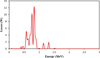 |
Fig. 6 Beam loss with respect to beam energy along the RFQ structure. |
 |
Fig. 7 Accelerated beam transmission along the RFQ structure. |
Optimized cell parameters and beam parameters of the RFQ.
 |
Fig. 8 Trajectory of the tune depression and phase advance ratio of the RFQ on the Hofmann chart. |
 |
Fig. 9 Initial coordinates of survived particles (blue color) over the input beam (black color). |
 |
Fig. 10 Beam transmission and output emittance as a function of input emittance. |
4 Error study
During the process of fabrication and alignment, various errors may get introduced in the RFQ cavity, e.g., profile error in the vane-tip and misalignment of vanes and sections. Also, there may be missteering and mismatch of input beam during injection in the RFQ. Effect of these errors on the beam dynamics can be rather large, which may result in an unacceptable beam quality. In order to ensure an acceptable output beam quality in the presence of various errors, we have derived the tolerances on different types of errors by performing a statistical error analysis using the beam dynamics code TraceWin, except for the voltage tilt error and voltage factor, for which the error calculation is performed with the code PARMTEQM. We have assumed a Gaussian distribution truncated at 3σ for the input beam and considered 105 macroparticles in our simulation. When we did not consider any error, the beam transmission efficiency was 97% and there was no growth in the transverse emittance. The longitudinal rms emittance at the RFQ exit was found to be 0.17 deg-MeV (0.45 mm-mrad).
In order to set the tolerance limit on the errors, we have to define an acceptable criterion for beam loss and emittance growth in the RFQ. Since the beam loss in RFQ may result in neutron generation and induced radioactivity, it is required that beam loss in RFQ is kept minimum. We define an acceptable limit of <2% for the additional beam loss due to errors, such that we have >95% beam transmission even in presence of various errors. A significantly higher emittance may also lead to beam loss, therefore, in order to limit the emittance of injector linac to twice that of the nominal case without errors, the additional emittance growth in RFQ due to errors was decided to be kept <10% [19].
The effect of combination of various errors was observed on the beam dynamics parameters of RFQ. Considering uniform distribution of errors within defined range with 1000 statistical simulations, the RFQ tolerances are specified in Table 3. With specified errors, the additional transverse and longitudinal rms emittance growth were found to be 7% and 3.4% respectively with beam loss of 1.6%.
RFQ error tolerances.
5 Electromagnetic design of RFQ cavity
Using the beam dynamics codes, the vane-tip parameters, i.e., the average aperture radius, transverse radius of curvature etc., were obtained, as described in the previous section. Next, the electromagnetic code SUPERFISH [20] was used to optimize the transverse cross-section geometry of the RFQ cavity. The design frequency of the RFQ cavity cross-section is chosen to be less than the operating frequency in order to keep a symmetric range for the tuners [21]. Tuners are used to tune the frequency as well as to correct the errors in the electromagnetic field, arising during mechanical fabrication and alignment process. Since tuners are more efficient inside the cavity than outside, their nominal position should be inside the cavity so that they can be moved in both the directions to correct the errors in an effective manner. Therefore, we had to design the transverse cross-section of the RFQ cavity at a lower frequency such that, when the tuners operate inside the cavity, the operating frequency of 325 MHz is restored. In our case, the two-dimensional (2D) cross-section of the RFQ was selected to be resonant at 319 MHz with tuners in flush position (zero position).
SUPERFISH is a 2D code and used to solve the symmetric structures only. RFQfish is a tuning program of SUPERFISH for RFQ and sets up the transverse geometry of the RFQ cavity such that it resonates at the desired frequency. RFQfish assumes a four-fold symmetry and therefore sets up SUPERFISH runs for only one quadrant of the RFQ. Figure 11 shows the outline of an RFQ quadrant set up by RFQfish and Figure 12 shows more details near the vane-tips [20]. The optimized geometrical parameters are shown in Table 4. The 2D transverse cross-section of the RFQ cavity has been kept constant along the RFQ length, in order to simplify the mechanical fabrication.
With these geometrical parameters, electromagnetic simulations were performed for a quadrant of RFQ. The fundamental quadrupole mode frequency of the cavity was optimized at 319 MHz, and the quality factor for this mode was calculated to be 10280. The dipole mode cut-off frequency was obtained as 310 MHz.
The total power dissipation on the walls per quadrant was 208 W/cm. Taking 30% safety margin for the practical situation, the structure power loss was calculated to be 377 kW. The beam power from the beam dynamics calculation was found to be 44.5 kW. The total power requirement in the RFQ is the sum of structure power dissipation and beam power, which will be 421.5 kW in this case. This is the peak value of RF power. For maximum 10% duty factor, the average RF power will be 42 kW. Also, the average structure power per unit length and the average structure power per unit area were calculated to be 10.8 kW/m and 0.83 W/cm2 only at 10% duty factor.
After the optimization of the vane-tip profile according to beam dynamics requirement, and optimization of the geometrical parameters of the transverse cross-section of the RFQ based on the 2D electromagnetic design, a 3D electromagnetic design study was performed using the 3D electromagnetic computer code CST-MWS [22].
Due to tight tolerances required on the machining of the vanes of a four-vane type RFQ, the full vane length of around 3.5 m cannot be machined in a single piece. Therefore, it is planned to divide the RFQ in three segments, then braze these segments to make a full length cavity. The RFQ accelerator accommodates various ports for different purposes, as shown in Figure 13. An RF port is needed for coupling the RF power to the RFQ from the RF source. In order to couple 421.5 kW of RF power from the indigenous solid state power sources, the coaxial loop type coupler is being designed. There will be a provision for 4 numbers of RF coupler ports distributed azimuthally symmetrical in the middle segment. Any type of port is a perturbation for the field in the cavity. Hence, by maintaining the symmetry of the ports in the four quadrants, we minimize the strength of the dipole mode excitation. The diameter of each of the RF port is chosen to be 80 mm according to the outer conductor diameter of the commercially available 3 1/8” coaxial cable for the loop type coupler. Typically, the vacuum level needed in the RFQ structure to avoid RF breakdown is ∼10−6 Torr [23]. For this purpose, the first and third segments contain the vacuum ports. There are total number of 8 vacuum ports, 4 in each segment, and distributed symmetrically around the four quadrants of the cavity. A provision of total 48 tuner ports is made available in the RFQ, distributed azimuthally symmetric in the RFQ cavity, to flatten the field inside the RFQ and to compensate for the frequency deviation due to any mechanical fabrication and alignment errors. In order to sense the field inside the RFQ, and for taking the feedback sample of the field for the control purpose, a total of 32 sampling loop ports are used along the length of RFQ.
 |
Fig. 11 Cross-section of one quadrant of an RFQ cavity. |
 |
Fig. 12 Details near the vane tips for the RFQ quadrant. |
Geometrical parameters of the RFQ.
 |
Fig. 13 The RFQ model with various ports. |
6 Tuning strategy
As discussed in the previous section, a total number of 48 tuner ports, each of 80 mm diameter are distributed symmetrically around the four quadrants, as shown in Figure 13. The tuners are metallic cylinders, which increase the frequency of the structure, when inserted in the quadrants. To be incorporated in the tuner ports, the tuner diameter is selected to be 78 mm, in order to account for the sufficient margin for the RF sealing.
In order to study the effect of tuners on the field profile and resonant frequency, we modelled the 3D geometry of RFQ cavity with unmodulated vanes in CST-MWS code. With tuners at flush position, the fundamental quadrupole mode frequency was calculated to be 318.99 MHz. The frequency shift of the RFQ due to insertion of the tuners in the range of −35 mm to +35 mm was calculated, which is shown in Figure 14. Also, the field flatness in the RFQ cavity was calculated with respect to the tuner positions, which is also shown in Figure 14. Error in the electric field flatness or electric field ripple is defined as 2(Emax − Emin)/(Emax + Emin), or ±(Emax − Emin)/(Emax + Emin), where Emax and Emin are the maximum and the minimum values of the transverse electric field, respectively, along the length of RFQ. It is clear from Figure 14 that the frequency and field error are very much sensitive to the tuners position, when the tuners operate inside the cavity volume. We observed that the frequency shifts linearly with the tuner position in the range of −5 mm to +35 mm. However, we have derived a limit of ±3% or 6% on the field ripple error using the code TraceWin for an acceptance criterion of less than 5% beam loss and less than 10% emittance growth, which limits the tuner position range to be [−5 mm, +20 mm]. In order to perform corrections on both sides of the cavity resonance peak, the tuners should be at about half of their tuning position range inside the cavity. Therefore, the nominal position of the tuners is selected to be +9.8 mm inside the RFQ cavity, at which the operating frequency of 325 MHz can be restored. With the specified range of tuner position, the tuning range of ±10 MHz can be achieved in our design.
To work as a resonator, the RFQ structure has to be closed at both ends, i.e., the entrance and the exit ends. However, if we close the RFQ ends by placing the conducting end-walls, the cut-off frequency of the quadrupole mode will correspond to TE211 mode instead of the desired TE210 mode. Therefore, the ends of the vanes of the RFQ structure should be shaped in such a way that the magnetic field of the fundamental quadrupole mode becomes tangential at the end-walls to satisfy the boundary conditions for the TE210 mode at the ends of the structure. These properly shaped vanes at the ends are called as vane-end cutbacks. Optimization of the cutback parameters is described in the following subsection.
 |
Fig. 14 Frequency shift and field flatness as a function of tuner position. |
6.1 Vane-end cutback design
A typical schematic of the vane-end cutbacks is shown in Figure 15. We have incorporated the variation of aperture in the RMS and FFS sections in our simulation model. The RMS and FFS sections were modeled in CST-MWS by translating the transverse vane profile curve towards the end-plates. Each translated curve, covered with PEC material, was shifted vertically (for vertical vanes) or horizontally (for horizontal vanes) according to the radial coordinates of vane-tip in the RMS and FFS sections, derived from the code VANES [4]. Then, the faces of the covered profiles were joined using loft operation in CST modeler in order to model the vane in the RMS and FFS sections. Various parameters need to be optimized for the design of cutbacks [24]. Here, b is the radius of the beam hole at the end-plate, t is the thickness of the end-plate, g is the gap between the vane and the end-plate, d is the undercut depth up to which the vane is removed, h2 and h3 are the heights of the vane at the starting and the end of the undercut respectively, and h1 is the full height of the RFQ vane from the beam axis. In the design, a slope of 45° is provided for the undercut on the vane to spread the power dissipation on the larger area. All these parameters were optimized such that the frequency of the vane-end cutback exactly matches the frequency of the operating quadrupole mode, i.e., 325 MHz. For optimization of the parameters at the entrance end and the exit end, we simulated the models of the first segment and the third segment, respectively. In these models, we ensured a flat field in the full segment in presence of the vacuum ports opening and the tuners insertion. The values of the optimized parameters of the vane-end cutbacks for both ends of the RFQ structure are listed in Table 5. The resonant frequency of the full length unmodulated RFQ cavity with cutbacks at both ends, opening of vacuum ports and the tuners insertion up to +9.8 mm was calculated to be 325 MHz with field ripple less than ±2% in the transverse electric field profile.
Next, we introduced the modulations on the vane-tips of the RFQ in accordance with the design data obtained from the code VANES. Perturbation due to these modulations on the field profile and frequency, and its correction using tuners are described in the following subsection.
 |
Fig. 15 Schematic of vane-end cutback. |
Parameters of the vane-end cutbacks.
6.2 Perturbation due to vane-tip modulations and its correction
In the presence of any local error, there will be a mixing of the field of HOMs with the unperturbed field of the operating mode. This mode mixing perturbs the field profile of the operating mode and the strength of perturbation is larger for a longer structure. We know that the fractional-field error in terms of the cavity resonant frequency shift δω0 caused by a delta-function error at some position z0 along the length of RFQ is derived as [2]
 where V0 is the unperturbed voltage, ω0 is the unperturbed resonant frequency, l is the length of the cavity and λ is the free space wavelength. In an RFQ, the modulation on the vane-tips can be considered as a perturbation, which may increase or decrease the local frequency. Therefore, an overall field tilt is obtained along the RFQ due to mixing of field component of HOMs, even with the designed modulation parameters without any error.
In order to study the effect of the vane modulations, we prepared a model of the RFQ with modulated vanes in the code CST-MWS. The process, which we have followed in order to create the modulations on the RFQ vane-tips, is being described below.
-
the longitudinal profile of vane-tip modulations for the horizontal pair as well as the vertical pair of vanes was generated using the program VANES [4] and this was saved as a text file, e.g., ‘*.txt’;
-
the transverse profile of vane-tip was modeled in CST-MWS using an arc. The points of arc were already derived from the beam dynamics design using the RFQ Design Codes [4], and the 2D cross-section optimization studies described in the previous section, using the code SUPERFISH;
-
the longitudinal vane-tip profile was imported in CST modeler from the text file ‘*.txt’;
-
the arc of transverse vane-tip profile was swept along the longitudinal vane-tip profile curve, which modeled the modulated vane-tip along the RFQ length. The vane-tip profile curves in the transverse and longitudinal planes are shown in Figure 16;
-
the same procedure was repeated for several additive small parts of the vane over the tip up to the vane-blank depth. After sweeping these parts along the modulation profile, all parts were added together to model the part of modulated vane up to the vane-blank depth, as shown in Figure 17;
-
remaining part of the vane above the vane-blank depth was generated by a polygon curve extruded up to the full length of the RFQ, and finally added with the part of vane modeled up to the vane-blank depth in order to model a full vane with modulated tips.
In this way, a full model of the RFQ with modulated vane profile was created using the code CST-MWS. The optimized vane-end cutbacks and the tuners inserted up to +9.8 mm were included in the RFQ model with modulated vanes. Using eigenmode solver of CST-MWS code, we calculated the resonant frequency and the field profile of the RFQ cavity. The field tilt due to modulations was calculated to be ±20% and is plotted in Figure 18. This field tilt is a result of the mixing of higher order quadrupole modes with the unperturbed operating mode due to perturbations present in the form of vane-tip modulations. Since we have not considered any misalignment or fabrication error in the model, and only a quadrant of the model was simulated with symmetry planes, the contribution of the higher order dipole modes in the perturbed operating voltage is neglected. The resonant frequency of the cavity was found to have reduced by 645 kHz due to effect of vane modulations.
The error in the field may be worse in presence of some machining and misalignment errors. Correction of this error in the field profile may become a serious issue in the case where the tuners operate at flush position. In that case, if one tries to flatten the field using the tuners, some of them may need to be inserted much deeper in the cavity volume, which would increase the resonant frequency significantly. Then, in order to compensate for the frequency error, all the tuners have to be retracted from the cavity volume; however, due to low efficiency of the tuners in the backward direction, as shown in Figure 14, the resonating frequency may not be restored at the operating value. In that situation, one has to go for a complex solution, e.g., to change the dimensions of the RFQ cavity cross-section in the magnetic field region near vane-base or in the electric field region near vane-tips etc. However, in our tuning strategy, where the tuners are designed to be inserted by +9.8 mm inside the cavity volume by default, we are able to correct the error in the field profile and resonating frequency using only the movement of tuners in forward as well as backward directions efficiently. We have successively increased the insertion depth of the tuners along the RFQ in order to compensate for the local frequency error produced by the vane-tip modulations. The required penetration depth of all the 12 tuners in a quadrant from the low energy end to the high energy end of the RFQ was found to be 9.8 mm, 9.8 mm, 9.9 mm, 9.9 mm, 10.2 mm, 10.2 mm, 10.5 mm, 10.5 mm, 11 mm, 11 mm, 11 mm and 11 mm, respectively. In this way, the field tilt error was reduced to be within ±3%, with resonant frequency recovered at 324.97 MHz, which is also shown in Figure 18.
In order to confirm the accuracy of the design process of vane-tip modulations in CST-MWS, and to check whether the tuned structure could generate the desired accelerating field, we have also compared the axial electric field derived from CST-MWS with that calculated by the RFQ design code PARI. The axial field profiles, normalized with the maximum value of the axial electric field, are plotted in Figure 19, which show a good agreement between the profiles.
In a practical RFQ, there may be various errors present in the structure, which would mix the components of higher order quadrupole as well as dipole modes in the operating mode. A study was performed in order to stabilize the operating mode against the mixing of HOMs, which is described in the following section.
 |
Fig. 16 Transverse and longitudinal profile curves of RFQ vane-tip. |
 |
Fig. 17 Few cells of modulated vane as seen from the high energy end of RFQ. |
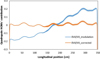 |
Fig. 18 Perturbative component of the quadrupole mode before and after correction. |
 |
Fig. 19 Axial electric field profiles calculated from CST MWS and PARI codes. |
7 Mode stabilization study
In a four-vane type RFQ, there are several undesired electromagnetic modes having frequency close to that of the operating mode. Most important are the dipole modes and the higher-order quadrupole modes. Due to the fabrication and misalignment errors, the operating mode gets perturbed by these nearby modes, and this has detrimental effect on the performance of the RFQ. The dipole modes can deflect the beam transversally, which will affect the beam transmission. On the other hand, the higher order quadrupole modes may give rise to an undesired variation in the longitudinal accelerating field along the length, which will affect the synchronization of the beam with the accelerating field, and hence may deteriorate the beam transmission. It is therefore desired that the operating mode is sufficiently separated in frequency from the undesired nearby modes.
7.1 Higher order mode spectrum
The dipole and quadrupole mode spectrum was obtained by solving the full length modulated RFQ model, tuned to minimize the perturbative component of higher order quadrupole modes, as described in the previous section. The mode spectrum can be seen in Figure 20.
The higher order quadrupole mode TE211 is nearest to the operating mode, and it is separated by +3.1 MHz from the operating mode. This is not too close to the operating mode to produce a significant undesired variation in the longitudinal electric field of the RFQ. However, the resonant coupling technique, proposed by Young [25], can be used to increase the separation of this mode from the operating mode. Due to the complexity of the resonant coupling scheme, it has been abandoned for the first trial of the fabrication process and the longitudinal field variation due to the higher order quadrupole mode will be compensated by the tuners only.
The neighboring dipole modes are the most dangerous for the operating field pattern inside the RFQ cavity. The dipole modes nearest to the operating mode are the TE111 mode on the lower side and TE112 mode on the upper side in the frequency spectrum. The separation of TE111 and TE112 dipole modes from the operating mode is calculated to be −2.8 MHz and +6.6 MHz respectively. Typical error during mechanical fabrication or alignment process can mix the field component of TE111 dipole mode to the field of the operating mode.
For the stabilization of the operating mode field against the mixing of the dipole field component, various techniques have been proposed, e.g., vane coupling rings [26], pi-mode stabilizing loops [27], DSR [28], etc. Being relatively simple to implement and effective as well, the DSR scheme has been chosen to provide a sufficiently wide and symmetric dipole mode free region around the operating mode to avoid the mixing of nearby dipole modes with the operating mode.
 |
Fig. 20 The mode spectrum of the RFQ structure. |
7.2 Dipole stabilization rods (DSRs)
DSRs are the cylindrical rods attached to the base of the end plates at the entrance and the exit ends. These are inserted longitudinally in each of the four quadrants to distribute the neighboring dipole modes symmetrically around the operating mode. In this way, the perturbation will tend to mix the nearby modes equally, but with opposite sign, with the operating quadrupole mode. Since these neighboring modes have similar characteristics, the effect of mixing one of these modes with the operating one is cancelled by the other mode. As a result, the field is better stabilized against perturbations [25]. The schematic of the DSRs inserted in each quadrant is shown in Figure 21. The main parameters of the DSR to be optimized are the diameter, the location and the penetration depth in the four quadrants.
The diameter d, and the radial location h of the DSRs in a quadrant of the RFQ, as shown in Figure 21, can be chosen by observing the frequency shift of the operating quadrupole mode. The criterion for the choice of the diameter of the DSRs is that it should be as small as possible so that it does not perturb the operating mode frequency, and it should have enough space for the cooling arrangement [28]. On the other hand, the location of DSRs is chosen at a particular point on the bisector of the quadrants such that the effect of perturbation on the electric and magnetic fields of the operating quadrupole mode cancel each other such that the frequency of the operating mode remains unperturbed [28]. The calculations were performed for various values of d; and for each value of d, a value of h was found such that the perturbation to the operating mode is minimum. Since the dimensions of vane-end cutbacks at both ends of the RFQ are different, the radial location of the DSRs at both ends are also different slightly. From 3D simulations, the optimum values were found as d = 14 mm, and h = 61.16 mm and 60.81 mm at the entrance end and the exit end respectively.
After determination of the diameter and the location of the DSRs, the optimum length of the DSRs that needs to be inserted in the quadrants, in order to ensure a sufficiently wide and symmetric frequency shift of the nearest dipole modes from the operating mode, was calculated. Calculation of the frequency shift of the nearby dipole modes, as a function of the length of the DSRs was performed using the computer code CST-MWS, and the results are shown in Figure 22.
The dipole mode excites the TEM-type bar modes in the quadrants [28], and due to these bar modes, energy is stored in the capacitance formed between the DSRs and the RFQ vanes. While inserting the DSRs up to vane-end cutback depth, the electric field, and hence, the capacitance between vane and DSR is rather small. As a result of this negligible capacitance between DSR and vane, the dipole mode frequencies remain almost unchanged. As it can be seen in Figure 22, up to around 5 cm insertion of DSRs, the frequency of all the dipole modes remains almost unchanged. As the DSR is inserted more deeply in the quadrants, the capacitance between DSR and vane increases, and consequently, the dipole mode frequencies decrease significantly. It is observed from Figure 22 that for a length of 15.5 cm of DSRs, the shift in the frequency of TE111 and TE112 modes from the operating mode, are −4.2 MHz and +4.3 MHz, respectively, which provides a sufficiently wide and symmetric frequency separation from the operating mode.
 |
Fig. 21 Schematic of the DSR in the quadrants of the RFQ. |
 |
Fig. 22 Variation of dipole mode frequencies with the length of DSRs. |
8 Conclusion
In the front-end of 1 GeV injector linac of ISNS project, an RFQ is a preferred choice to be used in the low energy regime, which efficiently bunches, focuses, and accelerates the 50 keV H− beam up to 3 MeV. The operating frequency of the RFQ was selected to be 325 MHz. Since the space-charge effects are very strong at the low energy end, the beam dynamics design of the RFQ is very crucial in order to provide a beam of good quality. The choice of beam dynamics parameters at the transition of the four sections of the RFQ, i.e., RMS, SH, GB and ACC, is a rather involved process. We have described the process in detail with necessary physical explanations. The nonlinear space-charge can introduce the parametric resonance instabilities in the high current RFQ linac. To avoid these instabilities, equipartitioning condition can be a choice in the design of RFQ. However, the equipartitioning is not a necessary condition to be followed. In our design of RFQ, we did not adopt the equipartitioning condition since it will make the design complex. Instead, we kept the value of tune depression ratio larger than 0.5 in the transverse as well as the longitudinal plane. In this condition, the tune points of the RFQ cross the instability resonance peaks, only where the growth rate of the instability is very weak. As a result of this, 99% particles get accelerated with less than 5% transverse emittance growth.
The transverse cross-section of the RFQ cavity was designed to resonate at 319 MHz, instead of the operating frequency of 325 MHz. This choice was adopted to gain maximum advantage of the tuners in both the directions of their movement. Since the beam dynamics codes do not consider the perturbation in the operating field due to vane-tip modulations, the 3D modelling of vane modulations using the code CST-MWS provides a platform to understand and overcome the effect of perturbation in the design stage itself. We calculated the error in the resonant frequency and field flatness due to vane modulations and corrected for this error by inserting successive tuners at varying depths. The HOM spectrum was calculated for the tuned RFQ cavity. The nearest quadrupole mode was found to be separated by +3.1 MHz from the operating quadrupole mode. We propose to compensate for the longitudinal field error, if any, due to mixing of this higher order quadrupole mode, by using the tuners only. The dipole modes, being deflecting in nature, are the most dangerous ones, and there should be sufficient separation in the frequency between the nearest dipole modes and the operating mode, for the stabilized operation of the RFQ. The separation of neighboring dipole modes to the operating mode was calculated to be −2.8 MHz and +6.6 MHz. We have planned to keep a provision of DSRs at both ends of the RFQ to make a sufficiently wide and symmetric dipole mode free region around the operating mode. Based on this design, including the tolerances derived from the error study, fabrication of a complete RFQ structure in three segments, each of around 1.15 m long is under progress.
Acknowledgments
We extend our thanks to Dr. S.B. Roy and Mr. S.C. Joshi for useful discussions, and Dr. P.A. Naik for his kind support and keen interest in the work. We would also like to thank Mr. Carlo Rossi from CERN and Mr. Olivier Piquet from CEA-Saclay for the useful conversation about the tuning procedure in the RFQ.
Author contribution statement
Rahul Gaur conceptualized the complete design problem, and performed the design calculations, along with analysis of results. Vinit Kumar conceptualized the beam acceptance calculation and tuning strategy discussed in Sections 3 and 6, respectively. Both authors, Rahul Gaur and Vinit Kumar, contributed to the preparation of manuscript.
References
- I.M. Kapchinskii, V.A. Teplyakov, Linear ion accelerator with spatially homogeneous focusing, Pribory Tekhnika Eksperimenta 119, 19 (1970) [Google Scholar]
- T.P. Wangler, Principles of RF Linear Accelerators ( John Wiley & Sons, New York, 1998) [Google Scholar]
- J.W. Staples, LBL-29472, Lowrence Berkeley Laboratory, University of California, Berkeley, California, 1990 [Google Scholar]
- K.R. Crandall et al., LA-UR-96-1836, Los Alamos National Laboratory, USA, 2005 [Google Scholar]
- http://irfu.cea.fr/Sacm/logiciels/index3.php [Google Scholar]
- N. Pichoff et al., Simulation results with an alternate 3D space charge routine, PICNIC, in Proceedings of 19th International Linear Accelerator Conference (Chicago, IL, USA, 1998), p. 141 [Google Scholar]
- W.E. Shoupp et al., Phys. Rev. 73, 421 (1948) [CrossRef] [Google Scholar]
- M. Ball et al., The PIP-II Conceptual Design Report, V0.00, 2017, http://pxie.fnal.gov/PIP-II_CDR/PIP-II_CDR_v.0.1.work2.pdf [CrossRef] [Google Scholar]
- R. Duperrier et al., Design of the ESS RFQs and chopping line, in Proceedings of XX International Linac Conference, TUD03 (Monterey, California, 2000), pp. 548–550 [Google Scholar]
- K.R. Krandall et al., LA-UR-79-2499, Los Alamos National Laboratory, USA, 1979 [Google Scholar]
- J.M. Han et al., Design of the KOMAC H+/H− RFQ Linac, in Proceedings of XIX International Linear Accelerator Conference (Illinois, 1998), pp. 774–776 [Google Scholar]
- B.G. Chidley et al., IEEE Trans. Nucl. Sci. NS-30, 3560 (1983) [CrossRef] [Google Scholar]
- Y. Kondo et al., PRST-AB 15, 080101 (2012) [Google Scholar]
- Zhihui Li, et al., PRST-AB 16, 080101 (2013) [Google Scholar]
- D. de Cos et al., Beam dynamics simulations on the ESS BILBAO RFQ, in Proceedings of 2011 Particle Accelerator Conference, MOODS6 (New York, USA, 2011) [Google Scholar]
- F. Gerigk, Beam halo in high-intensity hadron linacs, Dissertation for Doctor of Engineering, 2006 [Google Scholar]
- C.K. Allen, T.P. Wangler, PRST-AB 5, 124202 (2002) [Google Scholar]
- I. Hofmann et al., PRST-AB 6, 024202 (2003) [Google Scholar]
- M. Eshraqi et al., Statistical error studies in the ESS linac, in Proceedings of the 5th International Particle Accelerator Conference, THPME044 (Dresden, Germany, 2014) [Google Scholar]
- J.H. Billen, L.M. Young, LA-UR-96-1834, Los Alamos National Laboratory, USA, 2006 [Google Scholar]
- O. Piquet et al., The RF design of the LINAC4 RFQ, in Proceedings of IPAC'10, MOPD027 (Kyoto, Japan, 2010), pp. 738–740 [Google Scholar]
- CST Studio Suite, CST Microwave Studio, 2013, www.cst.com [Google Scholar]
- S. Shen et al., UCRL-JC-128065, Lawrence Livermore National Laboratory, 1997 [Google Scholar]
- R. Gaur, V. Kumar, JINST 9, T07003 (2014) [CrossRef] [Google Scholar]
- M.J. Browman, L.M. Young, Coupled radio-frequency quadrupoles as compensated structures, in Proceedings of 1990 Linear Accelerator Conference (Albuquerque, NM, 1990), pp. 70–72 [Google Scholar]
- H.R. Schneider, H. Lancaster, IEEE Trans. Nucl. Sci. NS-30, 3007–3009 (1983) [CrossRef] [Google Scholar]
- A. Ueno, Y. Yamazaki, Nucl. Instrum. Methods Phys. Res. A 300, 15 (1991) [CrossRef] [Google Scholar]
- F. Grespan et al., Nucl. Instrum. Methods Phys. Res. A 582, 303 (2007) [CrossRef] [Google Scholar]
Cite this article as: Rahul Gaur, Vinit Kumar, Beam dynamics and electromagnetic studies of a 3 MeV, 325 MHz radio frequency quadrupole accelerator, EPJ Nuclear Sci. Technol. 4, 9 (2018)
All Tables
All Figures
|
Fig. 1 Modulation parameter and peak surface electric field as a function of aperture radius for equal values of transverse and longitudinal current limits. |
| In the text | |
|
Fig. 2 Variation of beam dynamics parameters along the RFQ. |
| In the text | |
|
Fig. 3 Beam envelope in the transverse plane (upper) and longitudinal plane (lower). |
| In the text | |
|
Fig. 4 Normalized RMS emittances as a function of cell number along the length of RFQ. |
| In the text | |
|
Fig. 5 Halo parameter as a function of cell number in the RFQ structure. |
| In the text | |
|
Fig. 6 Beam loss with respect to beam energy along the RFQ structure. |
| In the text | |
|
Fig. 7 Accelerated beam transmission along the RFQ structure. |
| In the text | |
|
Fig. 8 Trajectory of the tune depression and phase advance ratio of the RFQ on the Hofmann chart. |
| In the text | |
|
Fig. 9 Initial coordinates of survived particles (blue color) over the input beam (black color). |
| In the text | |
|
Fig. 10 Beam transmission and output emittance as a function of input emittance. |
| In the text | |
|
Fig. 11 Cross-section of one quadrant of an RFQ cavity. |
| In the text | |
|
Fig. 12 Details near the vane tips for the RFQ quadrant. |
| In the text | |
|
Fig. 13 The RFQ model with various ports. |
| In the text | |
|
Fig. 14 Frequency shift and field flatness as a function of tuner position. |
| In the text | |
|
Fig. 15 Schematic of vane-end cutback. |
| In the text | |
|
Fig. 16 Transverse and longitudinal profile curves of RFQ vane-tip. |
| In the text | |
|
Fig. 17 Few cells of modulated vane as seen from the high energy end of RFQ. |
| In the text | |
|
Fig. 18 Perturbative component of the quadrupole mode before and after correction. |
| In the text | |
|
Fig. 19 Axial electric field profiles calculated from CST MWS and PARI codes. |
| In the text | |
|
Fig. 20 The mode spectrum of the RFQ structure. |
| In the text | |
|
Fig. 21 Schematic of the DSR in the quadrants of the RFQ. |
| In the text | |
|
Fig. 22 Variation of dipole mode frequencies with the length of DSRs. |
| In the text | |
Current usage metrics show cumulative count of Article Views (full-text article views including HTML views, PDF and ePub downloads, according to the available data) and Abstracts Views on Vision4Press platform.
Data correspond to usage on the plateform after 2015. The current usage metrics is available 48-96 hours after online publication and is updated daily on week days.
Initial download of the metrics may take a while.