© R. Kondo et al., Published by EDP Sciences, 2025

1. Introduction

Applications of Monte Carlo (MC) neutron transport calculation range from reactor analysis to high-fidelity multi-physics simulations. The challenges of the MC calculation become more apparent as the resolution of the calculation becomes higher. In the MC eigenvalue calculation, there are major two challenges in treating detailed distribution quantities such as flux or power distribution. One is the data size of the detailed distribution. Since a multi-physics simulation is one of the prime targets for obtaining detailed distribution quantities by the MC method [1–4], data transfer could be a bottleneck. The other is the statistical uncertainty of each value in a finely discretized tally region. Due to the nature of the MC calculation, many histories are required to reduce the statistical uncertainty of many small tally regions [2]. The functional expansion tallies (FETs) [5, 6] have been studied as one of the solutions for these challenges. In the FETs, a target distribution is expanded by orthogonal polynomials, e.g., Legendre [5–8] or Zernike polynomials [2, 9]. Expansion coefficients corresponding to the basic functions are tallied during the MC calculation. A continuous distribution can be obtained since the continuous basis functions are used. However, there are some issues with applying the FETs to practical problems. Firstly, applicable geometries are limited, e.g., one-dimensional line [5–8], disk [2], and sphere [9]. Secondly, the expansion order (equal to the number of expansion coefficients) could increase to represent a complex distribution [10, 11] since orthogonal polynomials do not consider the characteristics of the neutron transport calculation. To solve these issues, the flux distribution tallies using the proper orthogonal decomposition (POD) have been developed [11] as “the POD tallies”.

The dimensionality reduction using the POD [12] has been applied to neutronics calculations in recent studies [13–17]. In our previous study [11], the POD was applied to the spatial flux distribution in the MC eigenvalue calculation. In the POD approach, a target distribution is represented by a linear combination of orthogonal basis vectors. The singular value decomposition (SVD) is employed to extract the orthogonal basis vectors from snapshot data. To expand the target distribution with a small number of orthogonal basis vectors, snapshot data is chosen to capture the characteristics of the distribution. The dimensionality of a flux distribution is reduced from the number of spatial meshes in the distribution to the number of expansion coefficients. In the POD tallies, expansion coefficients are tallied during a random walk. The flux distribution is reconstructed after the MC calculation. The statistical uncertainty of the entire flux distribution increases monotonically with respect to the POD expansion order due to the methodological feature. Therefore, the statistical uncertainty of the flux distribution can be reduced if the POD expansion order is sufficiently low to represent the distribution.

The advantages of the POD tallies were verified compared with the conventional FETs in our previous study [11]. Dimensionality reduction and statistical uncertainty reduction were achieved in a one-dimensional heterogeneous whole core geometry by using the collision estimator. However, despite the potential of the POD tallies, our previous study left several aspects of the POD tallies, e.g., an implementation with a different estimator. Therefore, the objective of this study is to reveal several detailed characteristics of the POD tallies by employing a simple problem. In addition to the fundamental properties of the POD tallies, the following three topics are addressed. Firstly, a derivation of the POD tallies with the track length estimator is described. An implementation of the track length estimator is crucial for a problem including void or materials with small total cross sections. Results of implemented POD tallies with the track length and collision estimators are compared. Secondly, to investigate the impact of the statistical uncertainty of the snapshot data obtained by the stochastic method on the extracted basis vector, the deterministic and the stochastic methods for the snapshot calculation are compared. Finally, the impact of the covariances of the expansion coefficients on the variances of reconstructed flux distribution is investigated. Only variances of the expansion coefficients are required to estimate l²-norm based standard deviation as a global index of the entire flux distribution [11]. However, covariances of expansion coefficients are also required to estimate the local variances in the flux distribution. Even if the covariances of expansion coefficients are tallied, the computation cost is small with the low POD expansion order. This investigation is conducted to clarify whether the covariances of the expansion coefficients can be negligible.

This paper is organized into the following sections. In Section 2, an overview of the POD tallies and the implementation with the track length estimators are described. In Section 3, the results of the two different estimators and the characteristics of the POD tallies are discussed including a comparison between the deterministic and the stochastic method for the snapshot calculation, and the impact of the covariances of expansion coefficients on the statistical uncertainty of the expanded flux distribution. Section 4 summarizes the conclusions.

2. Method

2.1. Overview of the flux distribution tallies using the proper orthogonal decomposition

This subsection provided an overview of the flux distribution tallies using the POD [11], which is called “the POD tallies”. It is assumed that a target flux distribution with R discretized meshes $\overrightarrow{\varphi }$ can be expanded by N orthogonal basis vectors as follows:

$$\overrightarrow{\varphi }={\displaystyle \sum _{n=1}^N}{a}_n{\overrightarrow{u}}_n=\text{U}\overrightarrow{a},$$(1)

where

$$\overrightarrow{\varphi }={\left({\varphi }_1\cdots {\varphi }_R\right)}^{\text{T}},$$(2)

$$\text{U}=\left({\overrightarrow{u}}_1\cdots {\overrightarrow{u}}_N\right),$$(3)

$$\overrightarrow{a}={\left(a_1\cdots a_N\right)}^{\text{T}}.$$(4)

ϕ_r, ${\overrightarrow{u}}_n$ and a_n are the volume averaged flux in mesh r, the n-th orthogonal basis vector, and the n-th expansion coefficient, respectively. Since orthonormal basis vectors are used to expand the flux distribution, the expansion coefficients in Equation (1) can be written as follows:

$$\overrightarrow{a}={\text{U}}^{\text{T}}\overrightarrow{\varphi }.$$(5)

In the MC calculation, these expansion coefficients $\overrightarrow{a}$ are tallied. The target distribution is reconstructed by Equation (1) after the MC calculation. Statistical uncertainty of the reconstructed flux distribution is obtained from the covariance matrix of expansion coefficients $\text{cov}\left(\overrightarrow{a},\overrightarrow{a}\right)$ as follows [11]:

$$\text{cov}\left(\overrightarrow{\varphi },\overrightarrow{\varphi }\right)=\text{U}\mathit{cov}\left(\overrightarrow{a},\overrightarrow{a}\right){\text{U}}^{\text{T}}$$(6)

where

$$\text{cov}\left(\overrightarrow{\varphi },\overrightarrow{\varphi }\right)=\left(\begin{array}{ccc}\hfill \text{var}\left({\varphi }_1\right)\hfill & \hfill \dots \hfill & \hfill \text{cov}\left({\varphi }_1,{\varphi }_R\right)\hfill \\ \hfill ⋮\hfill & \hfill \ddots \hfill & \hfill ⋮\hfill \\ \hfill \text{cov}\left({\varphi }_R,{\varphi }_1\right)\hfill & \hfill \dots \hfill & \hfill \text{var}\left({\varphi }_R\right)\hfill \\ \hfill \hfill & \hfill \hfill & \hfill \hfill \end{array}\right),$$(7)

$$\text{cov}\left(\overrightarrow{a},\overrightarrow{a}\right)=\left(\begin{array}{ccc}\hfill \text{var}\left(a_1\right)\hfill & \hfill \dots \hfill & \hfill \text{cov}\left(a_N,a_1\right)\hfill \\ \hfill ⋮\hfill & \hfill \ddots \hfill & \hfill ⋮\hfill \\ \hfill \text{cov}\left(a_N,a_1\right)\hfill & \hfill \dots \hfill & \hfill \text{var}\left(a_N\right)\hfill \\ \hfill \hfill & \hfill \hfill & \hfill \hfill \end{array}\right).$$(8)

The diagonal component of $\text{cov}\left(\overrightarrow{\varphi },\overrightarrow{\varphi }\right)$ are the variances of the reconstructed flux distribution. As a global index of the statistical uncertainty of the reconstructed flux distribution, l²-norm based standard deviation of flux shown in Equation (9) is used [11].

$$\parallel {\sigma }_{\varphi }\parallel =\sqrt{{\displaystyle \sum _{r=1}^R}\text{var}\left({\varphi }_r\right)}=\sqrt{{\displaystyle \sum _{n=1}^N}\text{var}\left(a_n\right)}.$$(9)

l²-norm based standard deviation of flux is written by variances of expansion coefficients and increases monotonically with respect to the POD expansion order N. Therefore, if the target distribution can be expanded by a small number of the basis vectors, the statistical uncertainty of the reconstructed flux distribution can be reduced. The method described so far enables tallying the flux distribution and its uncertainty by using the basis vectors.

Orthogonal basis vectors are extracted from snapshot data by using the SVD in the POD approach. The multiple different calculation conditions for the snapshot data are prepared to extract basis vectors which can expand the target distribution well. These conditions are obtained by perturbing some parameters, e.g., atomic number density, albedo values of boundary [11, 16], or macroscopic cross sections [14]. The obtained snapshot data is aligned as the snapshot matrix as follows:

$$\mathrm{\varphi }=\left(\begin{array}{ccc}\hfill {\overrightarrow{\varphi }}_1\hfill & \hfill \dots \hfill & \hfill {\overrightarrow{\varphi }}_S\hfill \\ \hfill \hfill & \hfill \hfill & \hfill \hfill \end{array}\right)=\left(\begin{array}{ccc}\hfill {\varphi }_{1,1}\hfill & \hfill \dots \hfill & \hfill {\varphi }_{S,1}\hfill \\ \hfill ⋮\hfill & \hfill \ddots \hfill & \hfill ⋮\hfill \\ \hfill {\varphi }_{1,R}\hfill & \hfill \dots \hfill & \hfill {\varphi }_{S,R}\hfill \\ \hfill \hfill & \hfill \hfill & \hfill \hfill \end{array}\right),$$(10)

where S is the number of snapshot data. The SVD of the snapshot matrix extracts the orthogonal basis vectors U as follows:

$$\mathrm{\varphi }=\text{U}\mathrm{\Sigma }{\text{V}}^{\text{T}},$$(11)

where

$$\text{U}=\left({\overrightarrow{u}}_1\dots {\overrightarrow{u}}_S\right).$$(12)

Once the basis vectors are obtained, the expansion coefficients are tallied during the MC calculation based on Equation (5).

2.2. Implementation with the collision and the track length estimators

In this subsection, the implementation of the POD tallies with the track length estimators is newly described, besides those with the collision estimator provided in the previous study. If the cell tallies are used, the volume averaged flux of a mesh (tally region) r is tallied by the two estimators as follows:

$$\left(\mathrm{Collision}\hspace{0.5em}\mathrm{estimator}\right):{\varphi }_r=\frac{1}{V_r}\frac{1}{H}{\displaystyle \sum _{h=1}^H}{\displaystyle \sum _{k=1}^{K_{r,h}}}\frac{w_{r,h,k}}{{\mathrm{\Sigma }}_{t,r}},$$(13)

$$\left(\mathrm{Track}\hspace{0.5em}\mathrm{length}\hspace{0.5em}\mathrm{estimator}\right):{\varphi }_r=\frac{1}{V_r}\frac{1}{H}{\displaystyle \sum _{h=1}^H}{\displaystyle \sum _{p=1}^{P_h}}{w}_{r,h,p}{d}_{r,h,p}$$(14)

where V_r is the volume of the mesh r; h, k, and p are the indices of history, collision, and path length, respectively; H, K, and P are the number of histories, collisions, and path length, respectively; Σ_{t, r}, w, and d are the macroscopic total cross section of the mesh r, the weight of the history, and the path length, respectively. If the POD tallies are used, the n-th expansion coefficient a_n is tallied by substituting Equations (13) or (14) into Equation (5) as follows:

$$\begin{array}{cc}\hfill \left(\mathrm{Collision}\hspace{0.5em}\mathrm{estimator}\right):a_n& ={\overrightarrow{u}}_n^{\text{T}}\overrightarrow{\varphi }\hfill \\ \hfill & ={\displaystyle \sum _{r=1}^R}\left(u_{n,r}\frac{1}{V_r}\frac{1}{H}{\displaystyle \sum _{h=1}^H}{\displaystyle \sum _{k=1}^{K_{r,h}}}\frac{w_{r,h,k}}{{\mathrm{\Sigma }}_{t,r}}\right)\hfill \\ \hfill & =\frac{1}{H}{\displaystyle \sum _{h=1}^H}\left({\displaystyle \sum _{r=1}^R}\left({\displaystyle \sum _{k=1}^{K_{r,h}}}\frac{u_{n,r}{w}_{r,h,k}}{V_r{\mathrm{\Sigma }}_{t,r}}\right)\right),\hfill \end{array}$$(15)

$$\begin{array}{cc}\hfill \left(\mathrm{Track}\hspace{0.5em}\mathrm{length}\hspace{0.5em}\mathrm{estimator}\right):a_n& ={\overrightarrow{u}}_n^{\text{T}}\overrightarrow{\varphi }\hfill \\ \hfill & ={\displaystyle \sum _{r=1}^R}\left(u_{n,r}\frac{1}{V_r}\frac{1}{H}{\displaystyle \sum _{h=1}^H}{\displaystyle \sum _{p=1}^{P_h}}{w}_{r,h,p}{d}_{r,h,p}\right)\hfill \\ \hfill & =\frac{1}{H}{\displaystyle \sum _{h=1}^H}\left({\displaystyle \sum _{r=1}^R}\left({\displaystyle \sum _{p=1}^{P_h}}\frac{u_{n,r}{w}_{r,h,p}{d}_{r,h,p}}{V_r}\right)\right),\hfill \end{array}$$(16)

where u_{n, r} is the elements of the n-th basis vector in the mesh r. The POD tallies differ from the cell tallies only in that the values scored in each tally region are multiplied by the elements of the basis vector. Since the algorithm of the MC calculation is very similar between the POD and the cell tallies, the POD tallies are easy to implement in existing MC codes.

3. Results and discussion

3.1. Calculation conditions

A target flux distribution has one hundred meshes (width 0.1 cm) in a one-dimensional 10 cm slab geometry as shown in Figure 1. Both left and right boundary condition is vacuum. There are three materials in the slab geometry. One group MC calculation is carried out with macroscopic cross sections shown in Table 1. These macroscopic cross sections are obtained by the function of the continuous energy MC code MVP3 [18] with the compositions from the VERA benchmark problems [19].

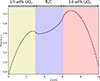Fig. 1. A target flux distribution.

To compare tally methods and estimators, the cell and the POD tallies with the collision and track length estimators are used with a one energy group in-house MC code. One hundred independent MC calculations are carried out to estimate real statistical uncertainty. As the reference calculations, the collision and the track length estimators of a multi-group MC code GMVP [18] are used with a large number of histories. The number of histories for each calculation is shown in Table 2.

The calculation conditions of snapshot data are prepared by separately perturbing the macroscopic cross sections of each material. All types of macroscopic cross sections are perturbed by the same fraction in a material. Giving four fractions, ±10, ±20% to each material in the slab, a total of 64 (= 4³) snapshot data is calculated before the MC calculation. Therefore, the snapshot matrix has 100 rows (the number of meshes in the flux distribution) and 64 columns (the number of snapshot data). The method of characteristics (MOC) is used to obtain the snapshot data by using the GENESIS code [20]. The calculation conditions for the MOC are shown in Table 3. Note that since the GENESIS code solves two-dimensional problems, the one-dimensional snapshots are obtained by solving two-dimensional geometry.

3.2. Snapshots and basis vectors

In this subsection, the prepared snapshot data and the extracted basis vectors are discussed before the MC calculation. Some examples of the snapshot data are shown in Figure 2, which are calculated by the GENESIS code with the calculation condition described in the previous subsection. By perturbing the macroscopic cross section of each material, various shapes of flux distributions can be obtained, varying the peaks of two kinds of fuels in the distribution. By preparing the snapshot data to capture the characteristics (variation) of the target distribution, the extracted basis vectors can reconstruct the distribution well.

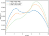Fig. 2. Examples of the flux distribution obtained by the GENESIS code (legends indicate the perturbation fraction of macroscopic cross section for each material, 3.1 wt.% UO2, B4C, and 3.6 wt.% UO2).

The deterministic method, the MOC, is used to obtain the snapshot data as described in the previous subsection. However, the possibility of using the stochastic method for the snapshot data should be discussed. To compare the extracted basis vectors between the deterministic and the stochastic method, additional snapshot calculations are carried out by the stochastic method with the GMVP code. The maximum standard deviation of the flux is less than 1% (using the collision estimator, the active batches: 1000, the inactive batches: 200, and the number of histories per batch: 10 000). The extracted basis vectors are shown in Figure 3. For the deterministic method, the first order basis vector is the average shape of the snapshot data. After the second order, the number of peaks and valleys in the basis vector increases with the order. On the other hand, the basis vectors of the stochastic method are degraded at higher orders. The shapes of the basis vectors of both methods are similar up to the third order. However, fine vibration gradually increases from the fourth order, and completely different shapes appear from the seventh order. This degradation of the basis vectors occurs because the SVD extracts the characteristics of the statistical uncertainty included in the snapshot data. Therefore, the statistical uncertainty of the snapshot data should be sufficiently small if the stochastic method is used. As for the snapshot calculation, the use of the deterministic method could be more efficient rather than that of the stochastic method with a large number of histories.

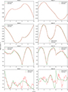Fig. 3. Basis vectors up to the eighth order extracted from the snapshot data obtained from the deterministic or the stochastic method.

3.3. Reconstructed flux distribution

In this subsection, the results of the MC calculation for the target flux distribution are discussed. Firstly, the tallied expansion coefficient and its relative standard deviation are shown in Figures 4 and 5, respectively. The statistical uncertainty is obtained from the mean values obtained from one hundred independent MC calculations. The absolute value of the expansion coefficient is large at lower order, as shown in Figure 4. This indicates that the lower order basis vectors are effective in reconstructing the target flux distribution. The expansion coefficients after the sixth order might be insignificant since their absolute values are small and their statistical uncertainty is relatively large. Comparing the collision and the track length estimators, the statistical uncertainty of the track length estimator tends to be smaller than that of the collision estimator in the first to the sixth order. As generally the case for the cell tallies, the track length estimator provides more precise results than the collision estimator for the POD tallies.

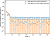Fig. 4. Tallied expansion coefficient (absolute value) with one standard deviation.

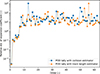Fig. 5. Relative standard deviation of expansion coefficient.

Secondly, the accuracy of the entire flux distribution is evaluated. As the global index of systematic error in the flux distribution, the root mean square error (RMSE) of Equation (17) is used.

$$\text{RMSE}=\sqrt{\frac{\sum _{r=1}^R{\left(\left({\overline{\varphi }}_r^{\mathrm{calc}}-{\varphi }_r^{\mathrm{ref}}\right)/{\varphi }_r^{\mathrm{ref}}\right)}^2}{R}},$$(17)

$${\overline{\varphi }}_r^{\mathrm{calc}}=\frac{1}{C}{\displaystyle \sum _{c=1}^C}{\varphi }_{r,c}^{\mathrm{calc}}$$(18)

where ${\varphi }_{r,c}^{\mathrm{calc}}$ is the flux in the mesh r obtained by the c-th independent MC calculation with the inhouse code, ${\varphi }_r^{\mathrm{ref}}$ is the flux in the mesh r obtained by the reference calculation, $R\left(=100\right)$ is the number of meshes (tally regions) in the flux distribution, and $C\left(=100\right)$ is the number of independent MC calculations with the in-house code. RMSEs with respect to the POD expansion order are shown in Figure 6. Note that the cell tallies do not depend on the POD expansion order since the flux itself is tallied. The POD tallies achieve the accuracy of the cell tallies at the sixth and the seventh expansion order. Therefore, the dimensionality of the flux distribution is reduced from one hundred to six for the collision estimator and seven for the track length estimator. For both the collision and the track length estimators, the RMSEs of the POD tallies decrease exponentially at lower order. They are below the RMSEs of the cell tallies and then asymptotically approach those of cell tallies. These trends occur due to decreasing truncation error and increasing statistical uncertainty. Note that RMSE includes statistical uncertainty since ${\varphi }_{r,c}^{\mathrm{calc}}$ is a result of the MC calculation. The order corresponding to the minimum RMSE for the track length estimator is higher (twelfth) than that for the collision estimator (seventh). This is because the increase in the statistical uncertainty of the POD tally for the track length estimator is smaller than that for the collision estimator, as explained later in Figure 7. This indicates that if the POD expansion order is the same, the track length estimator provides a more accurate result than the collision estimator.

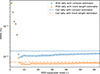Fig. 6. RMSE as systematic error with respect to the POD expansion order.

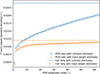Fig. 7. l2-norm based standard deviation with respect to the POD expansion order.

Finally, the statistical uncertainty of the flux distribution is evaluated. As the global index of statistical uncertainty in the flux distribution, l²-norm based standard deviation of Equation (19) is used.

$$\parallel {\overrightarrow{\sigma }}_{\varphi }\parallel =\sqrt{{\displaystyle \sum _{r=1}^R}{\sigma }_{{\varphi }_r}^2}=\sqrt{{\displaystyle \sum _{r=1}^R}\left(\frac{1}{C-1}{\displaystyle \sum _{c=1}^C}{\left({\varphi }_{r,c}^{\mathrm{calc}}-{\overline{\varphi }}_r^{\mathrm{calc}}\right)}^2\right)}.$$(19)

l²-norm based standard deviation with respect to the POD expansion order is shown in Figure 7. Note that the cell tallies do not depend on the POD expansion order since the flux itself is tallied. The l²-norm based standard deviations of the POD tallies increase monotonically. This feature allows the statistical uncertainty to be reduced if the POD expansion order is sufficiently low, as described in Section 2.1. The comparison between the POD and cell tallies is discussed. As shown in the above discussion of the systematic error with Figure 6, the sufficient expansion orders are the sixth and the seventh for the collision and the track length estimators, respectively. At these sufficient POD expansion orders, l²-norm based standard deviation of the POD tallies is reduced by 52% and 17% from those of the cell tallies for the collision and the track length estimators, respectively. The reduction in statistical uncertainty for the POD tallies with the track length estimator is smaller than with the collision estimator. The reason for this is that the present problem allows the track length estimator to score well and to obtain small statistical uncertainty for both the POD and the cell tallies since the mean free path (∼3 cm) could be relatively large for the geometry size (10 cm). The reduction of the statistical uncertainty might be larger in a problem with large geometry for the track length estimator. Comparing the POD tallies with the collision and the track length estimators, the l²-norm based standard deviation of the track length estimator is lower than that of the collision estimator, as shown in Figure 7. Consequently, the POD tally with the track length estimator can obtain a more precise solution is compared with the collision estimator.

3.4. Impact of the covariances of expansion coefficients on the expanded distribution

Only variances of the expansion coefficients are required to estimate l²-norm based standard deviation as a global index of the entire flux distribution. However, to estimate the variances of the reconstructed flux distribution, the covariance matrix of the expansion coefficients is required as described in Equation (6). If the impact of the covariances (i.e., the non-diagonal components in the covariance matrix) of expansion coefficients is negligibly small to the variance of flux, the computational resources could be reduced by ignoring the covariances. Therefore, an investigation is conducted to clarify whether only the variance components of the expansion coefficients can reconstruct the variances of the flux distribution. The variances of the flux distribution in the POD tallies are calculated by following three approaches. (a) “Reference”: the variance of the flux in each mesh is obtained by statistically processing the mean values of the reconstructed fluxes obtained from one hundred independent MC calculations with the POD tally. The covariances of the expansion coefficients and Equation (6) are not used. (b) Including covariances of expansion coefficients: the variances of the flux distribution are reconstructed with the covariance matrix of the expansion coefficients. (c) Excluding covariances of expansion coefficients: the variances of the flux distribution are reconstructed with only diagonal components in the covariance matrix of the expansion coefficients. Note that the POD tallies with the track length estimator at seventh order are used for all three results since the truncation error of the reconstructed flux distribution is sufficiently small, as mentioned in the previous subsection. The ratio of the relative standard deviation from the reference is shown in Figure 8.

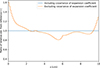Fig. 8. Ratio of the relative standard deviation including and excluding covariances of expansion coefficients from the reference (the POD expansion order is seventh).

If the covariances of expansion coefficients are used, the values coincide with the reference. On the other hand, if only the variances of the expansion coefficients are used, the values differ from the reference by a maximum of ∼60%. Therefore, not only the variances of the expansion coefficients but also the covariances of the expansion coefficients should be tallied to estimate the statistical uncertainty of the reconstructed flux distribution.

4. Conclusion

In this paper, the fundamental properties and characteristics of the flux distribution tallies using the POD are provided in the simple problem. The advantages of the POD tallies are the dimensionality and the statistical uncertainty reduction of the flux distribution compared with the cell tallies. In addition to showing these advantages as the fundamental properties of the POD tallies, some characteristics are revealed. Firstly, the POD tally is newly implemented with the track length estimator and is compared with the collision estimator. The track length estimator can obtain a more precise result for the POD tallies, similar to the cell tallies. Since the POD tallies reduce the statistical uncertainty by expanding the flux distribution with a small number of basis vectors, the POD tallies with the track length estimator are the most precise tallies among the present implementations. Secondly, the basis vectors obtained by the deterministic and the stochastic methods are compared. Since the snapshot data calculated by the stochastic method includes statistical uncertainty, the extracted basis vectors might be degraded. If the stochastic method is used for the snapshot data, a sufficient number of histories should be used to avoid degradation. Finally, the impact of the covariances of the expansion coefficients on the statistical uncertainty of the reconstructed flux distribution is investigated. Theoretically, the covariances of the expansion coefficients are required to estimate the variance of the local flux in a distribution. The flux variance reconstructed by only the variances of the expansion coefficients differs from the reference by ∼60% in the present simple geometry. This result indicates that the covariances should be included to properly estimate the statistical uncertainty of the reconstructed flux distribution.

In future work, there are two tasks as follows. One is an application of the POD tallies to a more practical problem. Specifically, a two- or three-dimensional geometry with unstructured meshes is in scope, such as a typical light water reactor. Since there are multiple identical fuel assemblies in the reactor, a more efficient dimensionality could be achieved by expanding flux distribution in different assemblies with the same set of basis vectors. These applications have already been applied for the deterministic method [15, 16]. An application with the MC method will be investigated with the POD tallies. If targeting a high-fidelity multi-physics simulation, a more finely discretized distribution should be solved, such as multiple fuel assemblies including fuel pins with radially several divisions. Another is to deal with underestimation of the statistical uncertainty of local tallies in the MC eigenvalue calculation [21]. To address this issue for the POD tallies, the real covariances of the expansion coefficients should be estimated to reconstruct the real variances of the expanded flux distribution. Since the FETs should also tally the covariances of the expansion coefficients corresponding to the basis function, the POD tallies and the FETs have similar concerns. However, the previous studies of the FETs have not clarified treating the covariance of expansion coefficients. It is worthwhile to investigate a methodology to estimate the real covariances of the expansion coefficients. A batch method [22] and circular block bootstrap method [23, 24] can be potential candidates due to their simplicity.

Funding

This work did not receive any specific funding.

Conflicts of interest

The authors have nothing to disclose.

Data availability statement

This article has no associated data.

Author contribution statement

Conceptualization, Ryoichi Kondo, Akio Yamamoto, and Tomohiro Endo; Methodology, Ryoichi Kondo; Software, Ryoichi Kondo; Formal Analysis, Ryoichi Kondo; Investigation, Ryoichi Kondo; Writing – Original Draft Preparation, Ryoichi Kondo; Writing – Review & Editing, Akio Yamamoto, and Tomohiro Endo.

References

All Tables

All Figures

	Fig. 1. A target flux distribution.
In the text

	Fig. 2. Examples of the flux distribution obtained by the GENESIS code (legends indicate the perturbation fraction of macroscopic cross section for each material, 3.1 wt.% UO2, B4C, and 3.6 wt.% UO2).
In the text

	Fig. 3. Basis vectors up to the eighth order extracted from the snapshot data obtained from the deterministic or the stochastic method.
In the text

	Fig. 4. Tallied expansion coefficient (absolute value) with one standard deviation.
In the text

	Fig. 5. Relative standard deviation of expansion coefficient.
In the text

	Fig. 6. RMSE as systematic error with respect to the POD expansion order.
In the text

	Fig. 7. l2-norm based standard deviation with respect to the POD expansion order.
In the text

	Fig. 8. Ratio of the relative standard deviation including and excluding covariances of expansion coefficients from the reference (the POD expansion order is seventh).
In the text

References

- K. Wang, S. Liu, Z. Li, G. Wang et al., Analysis of BEAVRS two-cycle benchmark using RMC based on full core detailed model, Prog. Nucl. Energy 98, 301 (2017), https://doi.org/10.1016/j.pnucene.2017.04.009 [CrossRef] [Google Scholar]
- M. Ellis, D. Gaston, B. Forget, K. Smith, Preliminary coupling of the Monte Carlo Code OpenMC and the multiphysics Object-Oriented simulation environment for analyzing Doppler feedback in Monte Carlo simulations, Nucl. Sci. Eng. 185, 184 (2017), https://doi.org/10.13182/NSE16-26 [CrossRef] [Google Scholar]
- A.J. Novak, D. Andrs, P. Shriwise, J. Fang et al., Coupled Monte Carlo and thermal-fluid modeling of high temperature gas reactors using Cardinal, Ann. Nucl. Energy 177, 109310 (2022), https://doi.org/10.1016/j.anucene.2022.109310 [CrossRef] [Google Scholar]
- T. Kamiya, T. Nagatake, A. Ono, K. Tada et al., Neutronics/thermal-hydraulics coupling simulation using JAMPAN in a single BWR fuel assembly, in Proceedings of the ICONE31 conference (Prague, Czech Republic, August 4–8, 2024), https://doi.org/10.1115/ICONE31-135974 [Google Scholar]
- W.L. Chadsey, C.W. Wilson, V.W. Pine, X-Ray photoemission calculations, IEEE Trans. Nucl. Sci. 22, 2345 (1975), https://doi.org/10.1109/TNS.1975.4328131 [CrossRef] [Google Scholar]
- D.P. Griesheimer, W.R. Martin, J.P. Holloway, Estimation of flux distributions with Monte Carlo functional expansion tallies, Radiat. Prot. Dosim. 115, 428 (2005), https://doi.org/10.1093/rpd/nci265 [CrossRef] [Google Scholar]
- D.P. Griesheimer, W.R. Martin, J.P. Holloway, Convergence properties of Monte Carlo functional expansion tallies, J. Comput. Phys. 211, 129 (2006), https://doi.org/10.1016/j.jcp.2005.05.023 [CrossRef] [Google Scholar]
- B.C. Franke, R.P. Kensek, Adaptive three-dimensional Monte Carlo functional-expansion tallies, Nucl. Sci. Eng. 165, 170 (2010), https://doi.org/10.13182/NSE08-68 [CrossRef] [Google Scholar]
- A. Jambrina, J. Leppänen, 3D Spherical Functional Expansion Tallies in Serpent 2 Monte Carlo Code, in Proceedings of the PHYSOR-2022 conference (Pittsburgh, PA, US, May 15–20, 2022) [Google Scholar]
- Z. Han, B. Forget, K. Smith, Using generalized basis for functional expansion, J. Nucl. Eng. 2, 161 (2021), https://doi.org/10.3390/jne2020016 [CrossRef] [Google Scholar]
- R. Kondo, T. Endo, A. Yamamoto, Flux distribution tallies using proper orthogonal decomposition in Monte Carlo calculations, J. Nucl. Sci. Technol. 61, 1536 (2024), https://doi.org/10.1080/00223131.2024.2365445 [CrossRef] [Google Scholar]
- J.S.R. Anttonen, P.I. King, P.S. Beran, POD-Based reduced-order models with deforming grids, Math. Comput. Model. 38, 41 (2003), https://doi.org/10.1016/S0895-7177(03)90005-7 [CrossRef] [Google Scholar]
- K. Tsujita, T. Endo, A. Yamamoto, Fast reproduction of time-dependent diffusion calculations using the reduced order model based on the proper orthogonal and singular value decompositions, J. Nucl. Sci. Technol. 58, 173 (2021), https://doi.org/10.1080/00223131.2020.1814891 [CrossRef] [Google Scholar]
- P. Behne, J. Vermaak, J.C. Ragusa, Minimally-invasive parametric model-order reduction for sweep-based radiation transport, J. Comput. Phys. 469, 111525 (2022), https://doi.org/10.1016/j.jcp.2022.111525 [CrossRef] [Google Scholar]
- K. Tsujita, T. Endo, A. Yamamoto, Efficient reduced order model based on the proper orthogonal decomposition for time-dependent MOC calculations, J. Nucl. Sci. Technol. 60, 343 (2023), https://doi.org/10.1080/00223131.2022.2097963 [CrossRef] [Google Scholar]
- M. Ito, T. Endo, A. Yamamoto, T. Takeishi et al., Reduced order SP 3 core calculation based on local/global iterations using proper orthogonal decomposition, J. Nucl. Sci. Technol. 62, 366 (2025), https://doi.org/10.1080/00223131.2024.2436958 [CrossRef] [Google Scholar]
- H. Chi, Y. Ma, Y. Wang, Reduced-order methods for neutron transport kinetics problem based on proper orthogonal decomposition and dynamic mode decomposition, Ann. Nucl. Energy 206, 110641 (2024), https://doi.org/10.1016/j.anucene.2024.110641 [CrossRef] [Google Scholar]
- Y. Nagaya, K. Okumura, T. Sakurai, T. Mori, MVP/GMVP version 3: General purpose Monte Carlo codes for neutron and photon transport calculations based on continuous energy and multigroup methods, JAEA-Data/Code 2016-018, (Japan Atomic Energy Agency, 2017) [Google Scholar]
- A.T. Godfrey, VERA Core Physics Benchmark Progression Problem Specifications, CASL-U-2012-0131-004, (Oak Ridge National Laboratory, 2014) [Google Scholar]
- A. Yamamoto, A. Giho, Y. Kato, T. Endo, GENESIS: A three-dimensional heterogeneous transport solver based on the legendre polynomial expansion of angular flux method, Nucl. Sci. Eng. 186, 1 (2017), https://doi.org/10.1080/00295639.2016.1273002 [CrossRef] [Google Scholar]
- K. Hayashi, T. Endo, A. Yamamoto, Underestimation of statistical uncertainty of local tallies in Monte Carlo eigenvalue calculation for simple and LWR lattice geometries, J. Nucl. Sci. Technol. 55, 1434 (2018), https://doi.org/10.1080/00223131.2018.1513875 [CrossRef] [Google Scholar]
- E.M. Gelbard, R. Prael, Computation of standard deviations in Eigenvalue calculations, Prog. Nucl. Energy 24, 237 (1990), https://doi.org/10.1016/0149-1970(90)90041-3 [CrossRef] [Google Scholar]
- D.N. Politis, J.P. Romano, A circular block-resampling procedure for stationary data, in Exploring the Limits of Bootstrap (Wiley, New York, 1992), pp. 263–270 [Google Scholar]
- L. Jin, K. Banerjee, S.P. Hamilton, G.G. Davidson, Improving variance estimation in Monte Carlo eigenvalue simulations, Ann. Nucl. Energy 110, 692 (2017), https://doi.org/10.1016/j.anucene.2017.07.016 [CrossRef] [Google Scholar]
Cite this article as: Ryoichi Kondo, Akio Yamamoto, and Tomohiro Endo. Fundamental properties and characteristics of flux distribution tallies using proper orthogonal decomposition, EPJ Nuclear Sci. Technol. 11, 21 (2025). https://doi.org/10.1051/epjn/2025019.