| Issue |
EPJ Nuclear Sci. Technol.
Volume 11, 2025
Status and advances of Monte Carlo codes for particle transport simulation
|
|
|---|---|---|
| Article Number | 4 | |
| Number of page(s) | 15 | |
| DOI | https://doi.org/10.1051/epjn/2024032 | |
| Published online | 24 January 2025 | |
https://doi.org/10.1051/epjn/2024032
Regular Article
Optimization progress of large-scale radiation shielding Monte Carlo simulation software based on AIS variance reduction technique system: MCShield
1
Department of Engineering Physics, Tsinghua University, Beijing, 100084, C.R. China
2
Key Laboratory of Particle and Radiation Imaging of Ministry of Education, Beijing, 100084, C.R. China
3
Nuctech Company Limited, Beijing, 100084, C.R. China
* e-mail: This email address is being protected from spambots. You need JavaScript enabled to view it.
Received:
11
June
2024
Received in final form:
8
November
2024
Accepted:
2
December
2024
Published online: 24 January 2025
Abstract
The development of novel nuclear facilities has brought safer and more efficient energy options but also poses significant challenges for radiation shielding calculations. MCShield, developed by the Radiation Protection and Environmental Protection Laboratory at Tsinghua University, is a Monte Carlo program designed for coupled neutron/photon/electron transport in radiation shielding calculations. It incorporates a system of variance reduction techniques based on Auto-Importance Sampling (AIS) to address the deep penetration problem commonly encountered in the field of radiation shielding. The accuracy and computational efficiency of MCShield have been validated through benchmark problems and real-world applications. However, the current AIS system faces limitations in complex scenarios, user-friendliness, and reliance on user experience. To address these issues, we optimized the size, shape, and energy parameters for the AIS variance reduction method, expanded the use of regular virtual surfaces, and introduced an irregular AIS virtual surface method. Additionally, we developed an automatic generation method for AIS virtual surfaces and implemented automatic calculation for these surfaces. AIS Energy Bias Method was proposed to improve convergence across different energy intervals. These improvements enhance the applicability and refinement of the AIS virtual surface parameters, significantly boosting the overall performance of MCShield.
© J. Wu, Published by EDP Sciences, 2025
 This is an Open Access article distributed under the terms of the Creative Commons Attribution License (https://creativecommons.org/licenses/by/4.0), which permits unrestricted use, distribution, and reproduction in any medium, provided the original work is properly cited.
1. Introduction
In the context of shielding design for nuclear facilities such as power plants, accelerators, and radiation apparatus, meticulous computation of radiation parameter distributions under various shielding schemes are imperative. Monte Carlo method, known is robust geometric representation, rapid convergence, and precise computational outcomes, has become the predominant technique for radiation field assessment in shield design endeavors [1]. However, this method encounters efficiency constraints when applied to complex geometrical configurations and deep penetration scenarios typical of primary and secondary radiation shielding calculation in advanced nuclear installations [2, 3].
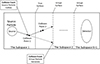 |
Fig. 1. Calculation flowchart of AIS method. |
The Radiation Protection and Environmental Protection Laboratory at Tsinghua University has developed a Monte Carlo program, MCShield, specifically designed for radiation shielding calculations involving coupled neutron/photon/electron transport, tailored to address various types of shielding challenges [4]. This program incorporates variance reduction technique system based on Auto-Importance Sampling (AIS) method, which has yielded favorable results [1, 5–8] on benchmark problems and real-world applications. AIS method divides the entire particle transport space into K + 1 sequentially adjacent subspaces by introducing virtual surfaces. The source particles are transported sequentially in layers between these subspaces. Through automatic particle weight adjustment and quantity control, the number of virtual particles on the virtual surface is equal to the number of source particles. The calculation flow of AIS method is illustrated in Figure 1.
However, in the shielding calculations for complex configuration nuclear facilities, AIS method faces several challenges:
-
a.
Insufficient Geometric Adaptability of Virtual Boundary Parameters: The regular virtual surface types currently employed in AIS method, such as planar, spherical and cylindrical surfaces, are inadequate for addressing the complexity of configurations in primary shielding. To better accommodate various geometric structures, it is necessary to enhance the geometric adaptability of virtual surfaces.
-
b.
Virtual Surface Setup Problem: Users often struggle to set up a suitable virtual surface for shielding calculation due to lack of experience. To address this issue, we propose an automatic generation method for different types of virtual surfaces, which facilitates the automatic calculation of AIS method.
-
c.
Convergence Issues in Energy Spectrum: Variance reduction computations require convergence across the energy spectrum, yet suboptimal convergence is observed in certain energy intervals. Current AIS methods lack the capability to adjust the energy space. Therefore, it is necessary to develop energy bias methods based on AIS to address the convergence issues in energy spectrum.
Below, we will discuss each of these issues in detail.
2. The description of optimization work
2.1. Geometric applicability amplification of AIS method
2.1.1. Amplification of regular AIS virtual surface method
The basic idea of AIS methods is to introduce virtual surfaces and to divide the computational space into several subspaces for hierarchical transport. The virtual surface is described by the following parametric equations:
 (1)
(1)
where u and v are parameters, and f(u,v) is a function of u and v. As depicted in Table 1, MCShield supports three regular virtual surfaces: planar, spherical and cylindrical surface. However, these regular virtual surfaces are only suitable for highly regular geometric scenarios and are inadequate for situations involving irregular core geometries, such as setting up hollow cylindrical surfaces or accommodating inclined surfaces. To address these limitations, we have expanded the regular virtual surface capabilities by:
-
(1)
Normal Direction Setting: Adding a normal property to set the normal direction of planar and cylindrical surfaces.
-
(2)
Hollow cylindrical surface Setting: Adding a cylinder inner diameter attribute for setting up hollow cylindrical surfaces.
Comparison of three types of regular virtual surfaces and their attributes.
These enhancements improve the flexibility and applicability of MCShield in handling complex geometric configurations. The specific diagram of comparison illustrating these enhancements is shown in Figure 2.
 |
Fig. 2. Geometric applicability expansion of planar and cylindrical virtual surfaces. (a) An inclined planar virtual surface (b) an oblique cylindrical virtual surface (c) a hollow cylindrical virtual surface. |
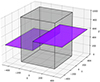 |
Fig. 3. Schematic diagram of an irregular AIS virtual surface composed of multiple planar virtual surfaces. |
2.1.2. Irregular AIS virtual surface method
In complex scenes, due to the strong anisotropy of geometry, it is often difficult to achieve optimal variance reduction results using a single regular virtual surface. Irregular AIS virtual surface method addresses this by generating virtual surfaces tailored to different geometric shapes based on a series of amplified regular virtual surfaces, as shown in Figure 3. Each virtual surface consists of several virtual sub-surfaces, which are spliced together to form a complete surface used for particle transport calculations. It can be described as a collection of a finite number of planar or cylindrical surfaces, each of which has its own parametric equation. We can represent their parametric equations as a set and ensure that they are correctly connected in space by appropriate conditions.
Supposing that there are N planar and M cylindrical surfaces with their respective parametric equations:
 (2)
(2)
Then the irregular AIS virtual surface can be represented as:
 (3)
(3)
When dealing with irregular virtual surfaces, there are notable differences compared to existing AIS methods. Each set of irregular virtual surfaces contains multiple virtual sub-surfaces, introducing additional complexity and adjustment requirements in terms of virtual surface input, construction, fast calculation, and inspection display in MCShield. To improve the efficiency and accuracy of constructing and searching irregular virtual surfaces, the MCShield team adopted a spatial binary tree method similar to the K-Dimensional tree (KDTree) [9, 10]. The KDTree is built recursively, sorting virtual surfaces according to depth and axis selection. At the leaf nodes, virtual surfaces are merged, and the root node of the KDTree is returned. This approach ensures efficient combination and management of each virtual sub-surface.
The calculation flowchart of irregular AIS virtual surface method (see Fig. 4) and specific schematics are outlined below.
-
(1)
Complete Monte Carlo modeling. The user introduces K irregular virtual surfaces, dividing the entire particle transport space into K + 1 sequentially adjacent subspaces. Each irregular AIS virtual surface Si is constructed based on several regular virtual surfaces Fi(ui,vi), where each irregular AIS virtual surface Si can be represented as Si = {Fi, j∪Fi, j + 1|1 ≤ i ≤ K}.
-
(2)
Sample source particles to obtain the source particle
 and initiate the transport calculation, where
  ,
,  , E, W are the direction of motion, position, energy and weight of the particle. After each collision, update the particle state
  . Determine if the particle can reach the current virtual surface position
  along with the direction
  .
. -
(3)
If the particle can reach the virtual surface and the position
 is in a region with non-zero importance, generate a pseudo-particle
  , and calculate and update the pseudo-particle weight
 .
. -
(4)
If the particle
 cannot reach the current irregular virtual surface Si along the direction
  , or if the position
  reached is in a region with zero importance, do not generate a pseudo-particle. When a source particle crosses the current irregular virtual surface Si to reach the next subspace,terminate it.
 -
(5)
Iterate steps (2), (3), and (4) until transport is completed for all virtual surfaces of thesubspaces.
-
(6)
Compute and output the results.
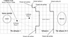 |
Fig. 4. Calculation flowchart of AIS irregular virtual surface method. |
 |
Fig. 5. Schematic diagram of automatic generation method of irregular AIS virtual surfaces. |
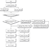 |
Fig. 6. Automatic calculation flowchart of AIS virtual surfaces. |
2.2. AIS automatic calculation method
2.2.1. Automatic generation method of irregular AIS virtual surfaces
Under simple geometric conditions of homogeneity, the automatic generation of AIS virtual surfaces is essentially a binary linear classification problem in 3D space, primarily handled by the Support Vector Machine (SVM) algorithm. The process involves finding the support vectors in the dataset to separate samples of different classes, maximizing the margin between them. This results in the best separating hyperplane with different penetration probabilities, which is used as the virtual surface. Due to the complexity of the geometry in the reactor space, it is not possible to achieve ideal computational results by using a single regular virtual surface. For this case, we divide the entire transport space into several grid cells of the same size and calculate the direct penetration probability of the center position of each cell with respect to the position of the source term. That is, the probability that the particle penetrates the current virtual surface without experiencing any collision event from the source term [4]. Based on the direct penetration probability of different positions, the surfaces of the grid cells are selected as an irregular virtual surface, as shown in Figure 5. The specific process of automatically generating irregular AIS virtual surfaces is as follows.
-
(1)
Complete the Monte Carlo geometric modeling, determine the statistical region R3, and divide the entire statistical region into Mx, My and Mz grid cells along the X, Y, and Z axes, respectively.
-
(2)
Calculate the direct penetration probability Pi, j, k for each grid cell Ni, j, k(1 ≤ i < Mx, 1 ≤ j < My, 1 ≤ k < Mz) in the entire transport space R3 is relative to the source term position
 , which is specified as:
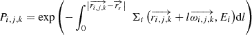 (4)
(4)
where
 is the direction vector of any position
  in space with respect to the source term
  ; Σt is the macroscopic total cross section, and Ei is the particle energy.
 -
(3)
Based on the penetration probability Ps of the cell Ns at the source term position
 , the penetration probability Pend, at the calculation boundary position
  , and the number of virtual surfaces K, determine the penetration probability threshold θi(1 ≤ i < K) for each subspace, ensuring consistent direct penetration probability within each subspace.
 -
(4)
Starting from the source term cell Ns, the direct penetration probability of the particle Pi, j, k at each cell Ni, j, k is calculated iteratively in layers. Judge whether Pi, j, k is greater than the threshold θi in the subspace, and record the index of the cell Ni, j, k.
-
(5)
After completing search for the current layer, select the outer surface of all recorded cells as the virtual surface for the current layer, removing overlapping parts with the source term cell Ns and the transport space R3 boundary to ensure the virtual surface is complete without omissions, and output the information of the virtual surface for the current layer as required.
-
(6)
Repeat steps (4) and (5) to ultimately complete the generation of K virtual surfaces.
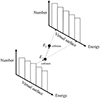 |
Fig. 7. Schematic Diagram of AIS Energy Bias Method. |
 |
Fig. 8. Schematic diagram of a multi-layer core water model. |
2.2.2. AIS automatic calculation method
Based on the above task, AIS automatic calculation method can be further implemented. It is important to note that MCShield uses five core classes to describe the whole particle transport process, from the top to the bottom: Simulation, Cycle, History, Route, and Step. The control relationship of the five classes is to be invoked layer by layer from the top to the bottom. Through the hierarchical structure of these classes, we are able to accurately simulate and control each step of the particle transport. The calculation process (see Fig. 6) is as follows:
-
(1)
Complete the Monte Carlo geometric modeling, initialize the program, parse the config and GDML files, and read the geometry, source term, statistical, material, and variance reduction information. If the user chooses to use AIS method, proceed to step (2); otherwise, proceed to step (9).
-
(2)
If the user chooses to automatically generate AIS virtual surfaces, proceed to step (3); otherwise, complete the AIS method initialization in MCShield and proceed to step (9).
-
(3)
Determine the statistical region R3, divide the entire statistical region into Mx, My and Mz cells along the X, Y, and Z axes, respectively, and calculate the direct penetration probability Pi, j, k for each grid cell Ni, j, k(1 ≤ i < Mx, 1 ≤ j < My, 1 ≤ k < Mz) in the entire transport space R3 is relative to the source term position
 .
. -
(4)
Based on the direct penetration probability Ps of the cell Ns at the source term position
 , the direct penetration probability Pend, at the calculation boundary position
  , and the number of virtual surfaces K, determine the penetration probability threshold θi(1 ≤ i < K) for each subspace, ensuring consistent direct penetration probability within each subspace.
 -
(5)
Starting from the source term cell Ns, the direct penetration probability of the particle Pi, j, k at each cell Ni, j, k is calculated iteratively in layers. Judge whether Pi, j, k is greater than the threshold θi in the subspace, and record the index of the cell Ni, j, k.
-
(6)
After completing the search for the current layer, select the outer surface of all recorded cells as the virtual surface for the current layer, removing overlapping parts with the source term cell Ns and the transport space R3 boundary to ensure the virtual surface is complete without omissions, and output the information of the virtual surface for the current layer as required.
-
(7)
Repeat steps (5) and (6) to ultimately complete the generation of K irregular virtual surfaces
 .
. -
(8)
Update the generated virtual surfaces in MCShield and complete the AIS method initialization.
-
(9)
Initialize the Simulation class and start particle transport, completing the History process for all particles, and recording statistical results during transport. If the user chooses to use AIS method, virtual particles are generated on the next virtual surface during particle transport, and automatic particle weight adjustment and quantity control are performed on the virtual surface.
-
(10)
After transport ends, output statistical results and terminate the program.
2.3. AIS Energy Bias Method
In Monte Carlo calculations, the relative statistical error in each region is determined by the number of particles entering the region, and the statistical errors varies accordingly to whether or not the simulated particles are uniformly distributed in different energy intervals [11]. In the actual Monte Carlo simulation, the theoretical analysis of relative statistical errors are more difficult because the statistics are more complex and may use geometric splitting and variance reduction techniques such as roulette and power windows, but the above conclusions are generally valid. Therefore, to meet the demand in practical engineering, i.e., to make all energy group calculations guarantee sufficient computational accuracy, we need to realize as much as possible that the particle distribution density of the particles in each energy group is uniform. To address these issues, the team proposed AIS Energy Bias Method. This method achieves a uniform distribution of virtual particles on the virtual surface within each energy group by employing an energy dimension control algorithm to regulate the number of virtual particles. Consequently, it ensures a uniform distribution of particles throughout the entire space of the Monte Carlo simulation for each energy group. Specifically, the energy dimension is added to the virtual surface, and the energy interval is divided. When adjusting the number of virtual particles on the virtual surface, the number of virtual particles generated is maintained within each energy interval. The technical scheme diagram of AIS Energy Bias Method (see Fig. 7) and the specific implementation process are as follows:
-
(1)
Introduce K virtual surfaces, dividing the entire particle transport space into K + 1 sequentially adjacent subspaces. For each virtual surface k, partition the energy dimension into G energy intervals.
-
(2)
Sample source particles to obtain the source particle
 and initiate the transport calculation. After each collision, update the particle state
  , and generate pseudo-particles on the virtual surface
  .
. -
(3)
Determine the energy interval g to which the pseudo-particle
 belongs to based on its energy Ei. If a particle reaches the current virtual surface during transport, terminate the particle.
 -
(4)
After completing transport within the current subspace, adjust the number of pseudo-particles Nk, g to maintain on the virtual surface k, energy interval g.
-
(5)
Pseudo-particles on the current virtual surface k act as source particles for the next subspace, and the transport process continues iteratively with steps (2), (3), and (4) until transport is completed for all virtual surfaces of the subspace.
-
(6)
Compute and output the results.
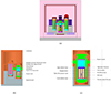 |
Fig. 9. Schematic diagram of the practical small reactor model. (a) Overall schematic diagram of the practical small reactor model. (b) Small reactor internals. (c) Small reactor core components. |
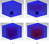 |
Fig. 10. Schematic diagram of four virtual surface settings. (a) No AIS. (b) Planar AIS virtual surfaces. (c) Cylindrical AIS virtual surfaces. (d) Irregular AIS virtual surfaces. |
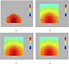 |
Fig. 11. Results of 3D neutron flux for four conditions. (a) No AIS. (b) Planar AIS virtual surfaces. (c) Cylindrical AIS virtual surfaces. (d) Irregular AIS virtual surfaces. |
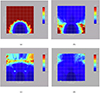 |
Fig. 12. Statistical errors of 3D neutron flux for four conditions. (a) No AIS. (b) Planar AIS virtual surfaces. (c) Cylindrical AIS virtual surfaces. (d) Irregular AIS virtual surfaces. |
3. Code validation test
After completing the code optimization work, the optimization module of MCShield was tested and verified. This paper presents tests on a multi-layer core water model and a practical small reactor model. It needs to be clarified that the statistical method mentioned in this paper is “Mesh Tally”. In this approach, the spatial distribution of physical quantities (e.g., neutron flux, dose rate, etc.) over the entire computational domain is obtained by dividing the computational domain into small virtual grid cells and counting the trajectories of particles in each cell.
3.1. Model A: A multi-layer core water model
The water model (see Fig. 8) is arranged in a multi-layer configuration, with the core located at the center of the lower bottom surface of the calculation space. The lower layer is wrapped with water, lead, polyethylene, and steel as shielding materials. The specific geometric parameters are as follows: the lower cylinder has a radius of 500 mm and a height of 400 mm, the upper cylinder has a radius of 400 mm and a height of 500 mm, the central water layer measures 2000 mm in length, 2000 mm in width, and 4000 mm in height, and the outer stainless-steel layer has a thickness of 1000 mm.
3.2. Model B: A practical small reactor model
The small reactor model consists mainly of a pressure vessel, steam generator, main pump, pressurizer, pipeline, suppression pool, and shielding structure. The pressure vessel is located at the center of the reactor chamber, as shown in Figure 9. Inside the pressure vessel are the fuel assembly, reflector, thermal shield, core basket, and other reactor inner structures. The core fuel assembly is modeled by homogenization. Various materials, such as stainless steel, lead, polyethylene, and water, are used as shielding structures around, above, and below the core. Neutrons and photons start from the fuel pellet, pass through the fuel assembly, reflector, pressure vessel, suppression pool, and other structures containing various shielding materials to reach the secondary shielding surface. In the small reactor model, the source term is a neutron source located in the core of a rectangular region (1 m long, 1 m wide, 2 m high, with the bottom center at the origin). The energy spectrum of the source term follows the Watt fission spectrum, and the direction is uniformly distributed.
4. Results
4.1. Irregular AIS virtual surface method: Model A
The effect of irregular AIS virtual surface method was tested using a multi-layer core water Model A. Five planar, cylindrical, and irregular AIS virtual surfaces were used, with the settings of the virtual surfaces are shown in Figure 10. The number of simulated particles was 107. The results (see Fig. 11) show that regular AIS virtual surface method cannot yield acceptable results. In the transport process of the planar AIS virtual surfaces, virtual particles are guided only upward, resulting in no calculation results around the core. For the cylindrical AIS virtual surfaces, because the lower core is closer to the side of the cylindrical AIS virtual surfaces, a large number of virtual particles are generated on the side, and fewer virtual particles are on the top, leading to abrupt changes in the flux results. In contrast, irregular virtual surface method can better conform to the shape changes of the core surface, resulting in more uniform neutron flux calculations across the entire space. The information about statistical error under different virtual surface conditions are compared (see Fig. 12 and Tab. 2). For the irregular virtual surfaces, the proportion of cells with the statistical error less than 5% was 35%, compared to 3% for the planar virtual surfaces and 26% for the cylindrical virtual surfaces, and the proportion of cells with the statistical error less than 15% was 67%, better than the planar ones (33%) and the cylindrical ones (47%).
Information about the statistical errors of different virtual surfaces.
To sum up, irregular AIS virtual surface method can achieve better results when calculating the same number of particles. This is mainly because the irregular virtual surfaces can more closely conform to the shape changes of different source terms, making it easier to obtain a more uniform particle spatial distribution and accurate radiation parameter calculation results. Compared to three types of regular virtual surfaces, irregular AIS virtual surface method offers certain advantages in more complex scenes.
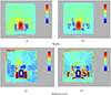 |
Fig. 13. Calculation results and statistical errors of regular AIS virtual surface. Results: (a) Y–Z plane (X = 0). (b) X − Z plane (Y = 0). Statistical errors: (a) Y − Z plane (X = 0). (b) X − Z plane (Y = 0). |
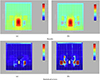 |
Fig. 14. Calculation results and statistical errors of irregular AIS virtual surface. Results: (a) Y − Z plane (X = 0). (b) X − Z plane (Y = 0). Statistical errors: (a) Y − Z plane (X = 0). (b) X − Z plane (Y = 0). |
4.2. AIS Automatic calculation method Model B
To evaluate the effect of the automatic calculation AIS method, a practical small reactor model was used for testing. The statistical range was −10 to 10 m in the X direction, −10 to 10 m in the Y direction, and −5 to 16 m in the Z direction, with a “Mesh Tally” cell size of 10 × 10 × 10 cm. The Figure of Merit (FOM) factor is used to evaluate computational efficiency, defined as:
 (5)
(5)
where T is the computation time and  is the average statistical error of the cell calculated as:
 (6)
(6)
where N is the number of cells in the full space and Ri is the statistical error within the ith cell.
Figures 13 and 14 show the neutron flux counting results and statistical errors of cells using regular cylindrical virtual surfaces and irregular virtual surfaces, respectively. It is evident that irregular virtual surfaces automatically generated achieve a lower and more uniform statistical error distribution compared to regular cylindrical virtual surfaces. Table 3 shows the calculation results and statistical errors of two virtual surfaces. The results indicate that the irregular virtual surface method can obtain better results with a particle count of 108 compared to the regular cylindrical virtual surface with 109 particles. Table 4 illustrates that the proposed irregular virtual surfaces described in this paper can achieve better computational performance.
Statistical errors of two virtual surfaces
Performance of two virtual surfaces.
Comparison of statistical errors of neutron spectra in different energy intervals.
4.3. AIS Energy Bias Method: Model A
The multi-layer core water model was used to test the effect of AIS Energy Bias Method. The energy intervals selected were 1.00E−05, 1.00E−03, 1.00E−01, 1.00E+00, 2.00E+00, 3.00E+00, 5.00E+00, 7.00E+00, 1.00E+01, 1.20E+01, and 1.50E+01 MeV. To verify the effect of AIS Energy Bias Method, the neutron fluxes of the full space for these energy intervals were calculated. Table 5 compares the statistical errors of the neutron flux across different energy intervals, with and without AIS Energy Bias Method. The table shows the proportions of cells with statistical errors less than 15% for a total of 1E+08 calculated particles. The results indicate that the statistical errors in the low energy region are generally similar in both cases, with the case without AIS Energy Bias Method performing slightly better. This is mainly due to the slowing down of source particles through the shielding material, causing the energy spectrum to shift to the low energy region, which aligns with physical laws. However, in the high-energy regions, the calculation results using AIS Energy Bias Method are significantly improved compared to those unbiased. In summary, AIS Energy Bias Method effectively enhances convergence across different energy intervals.
5. Conclusion
In recent years, the Radiation Protection and Environmental Protection Laboratory at Tsinghua University has proposed various variance reduction methods for global problems, source-detector problems, and regional problems. We have developed a variance reduction technique system based on AIS method, integrated into the Monte Carlo simulation software for large-scale radiation shielding, MCShield. Our team has recently improved and optimized the AIS system in three key areas: geometric parameters, automatic calculation, and energy parameters, addressing issues of insufficient applicability in complex scenes and ease of use.
For geometric parameters, regular AIS virtual surfaces method was extended by adding normal vector parameters for planar and cylindrical surfaces, as well as the setting of hollow cylindrical surfaces. Based on these enhancements, irregular AIS virtual surface method was proposed, along with the development of geometric construction and fast positioning methods.
In terms of automatic calculation of virtual surface, a method based on support vector machine was proposed, facilitating AIS automatic calculation method. Regarding energy parameters, AIS Energy Bias
Method was introduced, which divides the particle energy into different intervals and ensures a consistent number of particles across these intervals to improve convergence.
In summary, these optimization measures not only enhance the overall performance of MCShield but also improve its adaptability to varying conditions, making it more flexible and scalable for variance reduction calculations in complex scene structures in new nuclear settings.
Acknowledgments
We would like to extend our deepest gratitude to the Radiation Protection and Environmental Protection Laboratory at Tsinghua University for their invaluable support and guidance throughout this research. Additionally, we are grateful to our colleagues and collaborators, whose encouragement and assistance were instrumental in the completion of this study.
Funding
This work is supported by the National Natural Science Foundation of China (Key Program) (U23B2067, “Research on hybrid geometry automatic modeling and fast particle transport method for complex shielding problem”).
Conflicts of interest
Author WU Zhen is employed by Nuctech Company Limited. The remaining authors declare that the research was conducted in the absence of any commercial or financial relationships that could be construed as a potential conflict of interest.
Data availability statement
No data are associated with this article.
Author contribution statement
Jiajun WU: methodology, implementation, data curation, writing- original draft preparation. Zhen WU: data processing, technical validation, writing – review & editing. Ankang HU: conceptualization, resources, supervision, writing – review & editing. Yisheng HAO: software, supervision, writing – review & editing. Yanheng PU: supervision, writing – review & editing. Hui Zhang: supervision. Rui QIU: supervision. Junli Li: methodology, resources, writing – review & editing.
References
- S.S. Gao et al., Development of a radiation shielding Monte Carlo code: RShieldMC, in Proc. Int. Conf. Mathematics & Computational Methods Applied to Nuclear Science and Engineering (2017) [Google Scholar]
- Q. Zhang, L. Liu, Y. Xiao et al., Experimental study on the transverse mixing of 5×5 helical cruciform fuel assembly by wire mesh sensor, Ann. Nucl. Energy 164, 108582 (2021) [CrossRef] [Google Scholar]
- N.V. Hoffer, P. Sabharwall, N.A. Anderson, Modeling a helical-coil steam generator in RELAP5-3D for the next generation nuclear plant Idaho National Lab. (INL), Idaho Falls, ID (United States) [Google Scholar]
- J.L. Li et al., An auto-importance sampling method for deep penetration problems, Progr. Nucl. Sci. Technol. 2 732 (2011) [CrossRef] [Google Scholar]
- W. Xin, Research on key methods of High-efficiency radiation shielding Monte Carlo calculation and program development (Tsinghua University, Beijing, 2016) [Google Scholar]
- C.Y. Li, M.S. thesis, Tsinghua University, Beijing, 2008 (in Chinese) [Google Scholar]
- S.S. Gao, Ph.D. thesis, Tsinghua University, Beijing 2019 (in Chinese) [Google Scholar]
- S.S. Gao et al., Study on Monte Carlo Variance Reduction Method for Thick Shield and Small Detector Problem, Atomic energy science and technology Doi: 10.7538/yzk.2019.youxian.0371 (in Chinese) [Google Scholar]
- J. Du, F. Bian, A privacy-preserving and efficient k-nearest neighbor query and classification scheme based on k-dimensional tree for outsourced data, IEEE Access, 8, 69333 (2020) [CrossRef] [Google Scholar]
- R.F. Sproull, Refinements to nearest-neighbor searching ink-dimensional trees, Algorithmica 6, 579 (1991) [CrossRef] [Google Scholar]
- A.M. Ferrenberg, D.P. Landau, K. Binder, Statistical and systematic errors in Monte Carlo sampling, J. Stat. Phys. 63, 867 (1991) [CrossRef] [Google Scholar]
Cite this article as: Jiajun Wu, Zhen Wu, Ankang Hu, Yisheng Hao, Yanheng Pu, Hui Zhang, Rui Qiu, Junli Li. Optimization progress of large-scale radiation shielding Monte Carlo simulation software based on AIS variance reduction technique system: MCShield, EPJ Nuclear Sci. Technol. 11, 4 (2025) https://doi.org/10.1051/epjn/2024032

Jiajun Wu is currently a Ph. D. Candidate of Nuclear Engineering Department of Engineering Physics at Tsinghua University. Her research interests include Monte Carlo simulation and radiation dosimetry.

Zhen Wu is currently a senior engineer of Nuctech Company Limited. His research interests include Monte Carlo simulation, radiation dosimetry, accelerator radiation protection and medical radiation protection.

Ankang Hu is currently a postdoctoral researcher at Tsinghua University. His research interests include Monte Carlo simulation and modeling radiobiological effect.

Rui Qiu is currently a Professor at Tsinghua University. Her research interests include radiation dosimetry, accelerator radiation protection, medical radiation protection, Monte Carlo simulation, human body models and shielding technology.
All Tables
Comparison of statistical errors of neutron spectra in different energy intervals.
All Figures
|
Fig. 1. Calculation flowchart of AIS method. |
| In the text | |
|
Fig. 2. Geometric applicability expansion of planar and cylindrical virtual surfaces. (a) An inclined planar virtual surface (b) an oblique cylindrical virtual surface (c) a hollow cylindrical virtual surface. |
| In the text | |
|
Fig. 3. Schematic diagram of an irregular AIS virtual surface composed of multiple planar virtual surfaces. |
| In the text | |
|
Fig. 4. Calculation flowchart of AIS irregular virtual surface method. |
| In the text | |
|
Fig. 5. Schematic diagram of automatic generation method of irregular AIS virtual surfaces. |
| In the text | |
|
Fig. 6. Automatic calculation flowchart of AIS virtual surfaces. |
| In the text | |
|
Fig. 7. Schematic Diagram of AIS Energy Bias Method. |
| In the text | |
|
Fig. 8. Schematic diagram of a multi-layer core water model. |
| In the text | |
|
Fig. 9. Schematic diagram of the practical small reactor model. (a) Overall schematic diagram of the practical small reactor model. (b) Small reactor internals. (c) Small reactor core components. |
| In the text | |
|
Fig. 10. Schematic diagram of four virtual surface settings. (a) No AIS. (b) Planar AIS virtual surfaces. (c) Cylindrical AIS virtual surfaces. (d) Irregular AIS virtual surfaces. |
| In the text | |
|
Fig. 11. Results of 3D neutron flux for four conditions. (a) No AIS. (b) Planar AIS virtual surfaces. (c) Cylindrical AIS virtual surfaces. (d) Irregular AIS virtual surfaces. |
| In the text | |
|
Fig. 12. Statistical errors of 3D neutron flux for four conditions. (a) No AIS. (b) Planar AIS virtual surfaces. (c) Cylindrical AIS virtual surfaces. (d) Irregular AIS virtual surfaces. |
| In the text | |
|
Fig. 13. Calculation results and statistical errors of regular AIS virtual surface. Results: (a) Y–Z plane (X = 0). (b) X − Z plane (Y = 0). Statistical errors: (a) Y − Z plane (X = 0). (b) X − Z plane (Y = 0). |
| In the text | |
|
Fig. 14. Calculation results and statistical errors of irregular AIS virtual surface. Results: (a) Y − Z plane (X = 0). (b) X − Z plane (Y = 0). Statistical errors: (a) Y − Z plane (X = 0). (b) X − Z plane (Y = 0). |
| In the text | |
Current usage metrics show cumulative count of Article Views (full-text article views including HTML views, PDF and ePub downloads, according to the available data) and Abstracts Views on Vision4Press platform.
Data correspond to usage on the plateform after 2015. The current usage metrics is available 48-96 hours after online publication and is updated daily on week days.
Initial download of the metrics may take a while.