| Issue |
EPJ Nuclear Sci. Technol.
Volume 10, 2024
Status and advances of Monte Carlo codes for particle transport simulation
|
|
|---|---|---|
| Article Number | 10 | |
| Number of page(s) | 10 | |
| DOI | https://doi.org/10.1051/epjn/2024013 | |
| Published online | 11 October 2024 | |
https://doi.org/10.1051/epjn/2024013
Regular Article
An overview of last decade’s developments in RayXpert®, a 3D Monte Carlo code
TRAD – Tests & Radiations, 907 Voie L’Occitane, 31670 Labège, France
* e-mail: This email address is being protected from spambots. You need JavaScript enabled to view it.
Received:
11
June
2024
Received in final form:
26
July
2024
Accepted:
27
August
2024
Published online: 11 October 2024
Abstract
This article provides an overview of the developments made over the last 10 years within RayXpert®, a CAD-based geometry 3D Monte Carlo software developed by TRAD – Tests & Radiations. The main features of RayXpert® are its 3D Monte Carlo engine and its CAD-based geometry. It is also possible to import STEP file, automatically detect overlaps, and perform parallel Monte Carlo computations. During the last 10 years, numerous new features were added to the software: TTB approximation, dose and flux mapping, computation resumption, radioactive decay computation, script support, MPI computation, advanced convergence indicators, etc. New features such as advanced biasing or neutron-induced activation simulation are under development. This article presents the past and future functionalities of RayXpert®.
© N. Dray et al., Published by EDP Sciences, 2024
 This is an Open Access article distributed under the terms of the Creative Commons Attribution License (https://creativecommons.org/licenses/by/4.0), which permits unrestricted use, distribution, and reproduction in any medium, provided the original work is properly cited.
1. Introduction
RayXpert® [1] is a cross-platform (Windows, Linux) CAD (Computer-Aided Design) based geometry 3D Monte Carlo continuous energy computation code. The code was originally designed to perform shielding and radiation protection studies. It is developed at TRAD – Tests & Radiations by a dedicated team of developers and the programming language is C++. Although RayXpert® was launched in 2013, it is based on the mature software Fastrad® [2], released 20 years ago, which is also a CAD-based geometry 3D Monte Carlo code dedicated to dose deposition calculation in sensitive parts of satellites under space radiation environment. RayXpert® now has a lot of features in its last release (1.9.3) version that make the software more efficient for industrial use. Therefore, in the first part, the original functionalities of RayXpert® first release are presented. Next, the evolution of the software over the last decade will be described. Finally, the prospective new features of the next versions of RayXpert® are introduced.
2. Original features of RayXpert®
2.1. Geometry definition
Numerous 3D Monte Carlo computation codes exist today [3], such as MCNP6.2 [4], TRIPOLI-4 [5], SCALE [6], Geant4 [7] or FLUKA [8]. All of these codes have geometry definition based on Constructive Solid Geometry (CSG). On the other hand, RayXpert® [1] has a boundary representation (B-Rep) geometry definition. This allows to model complex geometrical elements that cannot be produced by CSG. Moreover, as the B-Rep is used, STEP files [9] can be used to directly import geometrical shapes in the model. Another advantage of this type of geometrical representation is that it is not necessary to define a world cell. Finally, all the geometry definition is CAD-based and embedded in a modern Graphical User Interface (GUI) where all the model parameters can be defined. Figure 1 shows a screenshot of RayXpert® GUI with a STEP imported geometry.
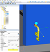 |
Fig. 1. Screenshot of the RayXpert® GUI with a STEP imported geometry example. |
Through the use of the B-Rep of the geometry, RayXpert® can compute the location and shape of overlaps and provide options to automatically correct them. It is a critical feature (that is not available in all Monte Carlo codes) since uncorrected overlaps can yield incoherent results.
2.2. Available particles
Initially, RayXpert® was designed to perform shielding and radiation protection calculations. The particle physics was based on Geant4 [7] physics. The available particles were photons, electrons, and positrons. Table 1 gives the photon processes [10, 11] handled in RayXpert® and the energy range of each process.
Photon processes handled in RayXpert® and energy range of each process.
In the same way, as for the photons, Table 2 gives the electron processes [10, 11] handled in RayXpert® and the energy range of each process.
Electron processes handled in RayXpert® and energy range of each process.
Finally, the positron processes supported by RayXpert® and the energy ranges are the same as those for electrons given in Table 2 with the addition of the annihilation process [10, 11], available from 1.022 MeV to 100 GeV.
2.3. Source definition
The first release of RayXpert® (in 2012) had two different types of sources. The first one called “continuous spectra” is basically a fixed source defined by the user. Every component of the source distribution is determined by the user and primary particles are sampled from this distribution. The other source type is called “radioactive decay”. The user selects a radio material, which has an associated decay spectrum. A radio-material is characterized by a list of radioactive isotopes with their activity fraction in the material. The user can also specify secular equilibrium [12, 13] for all or some of the radio-isotopes selected. It is essential to take into account radioactive filiation in some cases, such as 137Cs whose daughter isotope 137mBa produces the predominant decay rays (662 keV). Secular equilibrium thus allows considering the activity of the daughter nuclei simply by adding the parent nucleus. The user then has to specify the source direction and origin (volume or surface of a given geometrical element). Finally, the decay rays can be filtered by intensity and particle type in order to improve computation efficiency.
2.4. Parallelism
As RayXpert® is completely developed in C++, Monte Carlo computation could be fully parallelized through the use of OpenMP [14]. The only input needed from the user is the number of threads to use. The maximum thread count available was therefore equal to 64 due to OpenMP threads count limitation. Nevertheless, parallelism still allows us to improve significantly the Monte Carlo computation efficiency.
3. Last decade developments
So far, only the available features of the initial release of RayXpert® have been presented. However, lots of new functionalities were introduced in the software during the last decade. The next part of the article is therefore focused on the description of the more important ones.
3.1. TTB option
The simulation of electrons in a Monte Carlo computation is a highly consuming process in terms of numerical resources due to the amount of interactions of electrons in matter. To improve the Monte Carlo calculation efficiency involving electron transport, the Thick-Target Bremsstrahlung approximation [15–17] was introduced in RayXpert® 1.2 in 2013. This option disables secondary electron tracking during photon transport in matter. Instead, it is assumed that the electrons are locally slowed to rest and the photons from the Bremsstrahlung process are created in the same direction as the electron they replace. Therefore, a lot of electrons are not tracked resulting in a better computation performance while having a negligible impact on scoring results.
3.2. Mapping
Another useful feature that has been integrated into RayXpert® is the support of result mapping. The first iteration of this feature was a simple 3D Cartesian mesh, that was added in 2015 in RayXpert®. Then, more recently, both the support of 3D cylindrical and 3D tetrahedral meshes were added to the software in 2023, with the release of RayXpert® 1.9. Triangular and rectangular 2D surface meshes have also been implemented. Figures 2 and 3 show respectively the photon flux results obtained over a 3D Cartesian mesh and a tetrahedral mesh generated with RayXpert®.
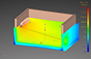 |
Fig. 2. Photon flux results obtained on a Cartesian mapping with RayXpert®. |
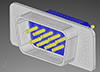 |
Fig. 3. Example of tetrahedral mapping generated with RayXpert®. |
A dedicated post-processing interface is also available. More precisely, Figure 2 shows the post-processed results of the Monte Carlo computation in RayXpert®. This interface also has options to filter results using uncertainty (shows only the result with sigma below a user-defined threshold value), cut the view, display results as slice, change the results scale (logarithmic, linear, or root square), etc. A zoning tool changes the way RayXpert® displays this information. Instead of a continuous display of values, they are grouped into ranges, which can allow the user to quickly identify areas where the dose rate is higher than a given threshold. This tool is often used to highlight controlled/restricted areas based on the specific local ruling of nuclear safety authorities.
3.3. Computation resumption
When running a Monte Carlo computation, it is impossible to know beforehand the simulation time (or the number of primary particles) needed to obtain the desired error level in the detector. Thus, a computation resumption feature has been developed in RayXpert® during the last decade. When requested, a resumption file is generated during the Monte Carlo calculation. This file can then be loaded into RayXpert® to resume the computation, adding more time (or more new primary particles) to the simulation as requested. It is also possible to resume several times in a row a computation.
3.4. Dose computation
RayXpert® was initially developed for shielding and radiation protection studies. Afterward, flux-to-dose coefficient factors were added for a score computation. Indeed, the user can now select score from the defined list for any detector or mesh defined. H*(10) coefficients [18], E(AP), E(ISO) [19], and other coefficients from ICRU57 [20] are available and directly taken into account to yield the desired score. Air and water Kerma [21] are also included. Table 3 lists the new quantities added to RayXpert®, version by version.
Quantities added to RayXpert®, version by version.
3.5. Weight window biasing
In radiation protection and shielding studies, it is common to require long runtime. Indeed, these studies aim to design well-shielded facilities. Therefore, the flux attenuation is important in these cases. So, very few particles reach detectors and convergence is slow. To improve Monte Carlo computation efficiency, a weight window biasing method [17] has been integrated to RayXpert® in 2016. Cell weights are calculated by considering the attenuation of photons in a straight line between each source and each detector. When a particle passes through a material, the coefficient of attenuation is equal to the concrete coefficient weighted by the material density. Then the particle undergoes either Russian roulette or splitting, depending on its weight with respect to the cell’s weight during transport. Even though the method used to calculate the weight windows is rough, in most cases it improves significantly Monte Carlo calculation efficiency.
3.6. Script
In many cases, setting up a simulation can involve a lot of repeated tasks. For example, running sensitivity studies requires generating numerous models with slight variations. Another current example in radiation protection studies is when fuel rod assembly storage is modeled. Indeed, the user has to place every fuel rod and assembly. For any repetitive task, the script feature is well suited. In RayXpert®, an integrated script functionality was added in 2017. The script engine is based on the ChaiScript language [22] and allows it to interact with most parts of the software.
3.7. Distributed computation
By construction, the Monte Carlo computation principle is to simulate particle histories to compute detectors scores. In many cases, it is required to launch a huge amount of primary particles to reach acceptable results accuracy. Even if RayXpert® has a built-in parallelism feature, the maximum thread count is limited to 64 due to OpenMP. To overcome this limitation, a distributed version of RayXpert® has been developed in 2018. This version uses the Message Passing Interface (MPI) protocol [23, 24] to increase the maximum number of threads available for Monte Carlo computation. Using MPI, it is then possible to launch RayXpert® in an HPC (High-Performance Computing) center and to drastically reduce the simulation duration (in terms of elapsed time).
3.8. Advanced convergence indicators
As previously said, particles transport is the basis of Monte Carlo simulation. It is easy to understand that to obtain a result, particles must reach the detectors. Similarly, the greater the number of particles that reach the detectors, the more precise the results will be. More precisely, since all source particles are independent of each other and their histories are obtained using the same probability laws, according to the central limit theorem [25], if the number of simulated particles is large enough, the scores samples should follow a normal distribution. Hence, for each Monte Carlo calculation result, there is a purely statistical error coming from the method itself. To ensure results consistency, several convergence indicators have been implemented in RayXpert®. Assuming a result follows a normal distribution, it should become stable over the course of the calculation and the statistical error should decrease and adjust according to the  law (where N refers to the total primary particles simulated). These are 2 examples of convergence indicators available in RayXpert®. The details of the 7 convergence indicators available in RayXpert® are given in [1]. It is important to note that all convergence indicators must be fulfilled to accept result but it is not proof that the result is correct. It involves that if any of the convergence indicators is not reached, then the result should not be accepted.
3.9. Neutron transport
Initially, RayXpert® was developed for shielding studies, which tend to be photon and electron based. Nevertheless, neutrons and neutron sources are relatively commonplace in the nuclear industry. Therefore, neutron transport and interaction have been added to the software in 2018 for the 1.7.0 release of RayXpert®. ENDF/B-VII.1 [26] nuclear data post-processed at 293.6 K by PREPRO2015 [27] are used to compute interaction probabilities and neutron track length between 10−11 MeV and 20 MeV.
3.10. Time decay
Sometimes, secular equilibrium is not accurate enough to fairly represents the source term of the simulation. It can also be interesting to monitor the evolution of a source term and its zoning requirement for a period of time. For these situations, a time decay solver has been implemented in RayXpert® in 2016. This feature computes the inventory at the requested time of a radioactive material by solving the Bateman equations [28]. This new source term can be used in a calculation or automated calculations can be launched for the different time steps. A file containing the activity and quantity of each nucleus is also generated. For example, starting from a chemically pure 238U lump, secular equilibrium can bring an increase in total activity of about a factor 3. Figure 4 shows the time decay solver results obtained with RayXpert® for the lump of 238U, which can help the user visualize the evolution of its sources and can generate RayXpert®’s models at the different time steps.
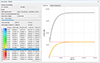 |
Fig. 4. Time decay solver results obtained with RayXpert® for the lump of 238U. |
3.11. Pulse height scoring
Pulse height scoring was added in RayXpert® 1.5.3 in 2017. This specific application case is designed to track the energy deposited in a detector by a particle. The user can specify Gaussian Energy Broadening (GEB) coefficients in order to replicate the response of a physical detector. This enables RayXpert® to be used to calculate efficiency curves, and model gamma spectrometers and helps in the design of new equipment. Figure 5 shows the difference between a score with GEB and a score without GEB, using a 192Ir source and GEB parameters from a typical NaI detector.
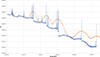 |
Fig. 5. Pulse height score for 192Ir spectrum with (orange) and without (blue) GEB. |
3.12. Versioning and read-only
Even if RayXpert® is a software well suited for research and education, it is mainly dedicated to industry. For such a context, versioning and read only mode were introduced in RayXpert® 1.9. Versioning allows to track any model modification. It can be used to perform audits, check implementation, or provide accountability. Read-only mode locks the model to prevent any accidental modifications or to provide additional safety for sensitive models.
3.13. S(α, β) and temperature effect
When a material is defined in a model, each isotope has to be declared. In specific application case, it can be important to specify not only the isotopic composition of the element, but also the molecular composition (H in H2O, or (CH2)n, or ZrH, ...) as it could impact results. S(α, β) coefficients [29] then have been integrated in RayXpert® to take into account molecular effects. Temperature effects (from 1.0 K to 1800.0 K) have also been taken into account.
3.14. Validation folder
To verify and test the proper integration of the various physical models in RayXpert®, multiple simulations have been performed in order to check and verify that the results are correct. The current validation folder includes 13 validation files on different subjects:
-
8 validation files on H*(10) calculation in different scenarios covering a range of application (shielding, radionuclides, self-attenuation, build-up effects),
-
2 validation files on neutron flux comparison with other codes [30, 31],
-
1 validation file on Bremsstrahlung rate of production as a function of angle which include comparison with experimental data [32],
-
1 validation file on the decay solver through a comparison with the benchmark described in [33],
-
1 related to a code-to-code comparison of HPGe detector modeling and GEB validation.
4. Future developments
Last decade of developments has made RayXpert® a powerful and suitable tool for Monte Carlo-based calculations applied to radiation and shielding studies. However, RayXpert® keeps getting improved based on both user feedback and developments meant to reach new user bases. Currently, RayXpert® supports electrons, positrons, photons and neutrons. Moreover, no advanced automated biasing methods are available in release version. Therefore, new functionalities are being under development to improve RayXpert®’s efficiency and open up its field of application. In the next section, we will discuss these improvements which will be available in the next software releases.
4.1. Importance map generation
First of all, a built-in Importance Map (IM) [34, 35] generator is under development in RayXpert. This importance map generator is only compatible with neutrons and photons. A few parameters are needed to generate an IM: particle type, energy binning, mesh definition and attractors list. An attractor is a cell towards which the user wants to direct the particles. The importance is a dimensionless value that approximately characterizes the expected contribution probability of particles located in the phase space position ( ) to the attractor. Figure 6 gives an example of the photon importance map generated with RayXpert® between 32.0 keV and 1.0 MeV for the geometry presented in Figure 2.
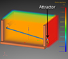 |
Fig. 6. Example of the photon importance map generated with RayXpert® between 32 keV and 1.0 MeV for the geometry presented in Figure 2. |
From Figure 6, it is possible to see that importance is the highest next to the attractor and the lowest in the roof of the room (for visibility reasons, roof is hidden in both Figures 2 and 6). The importance map obtained is therefore consistent with expectation. Indeed, the contribution of particles located in the roof should be lower than others as these particles have to go through two walls to reach the attractor. Moreover, the importance next to the attractor (on the right in Fig. 6) is the highest as there is only air in this part of the model. Therefore, it seems that IM generated with RayXpert® for this particle type and this model is consistent with expectation.
4.2. New advanced convergence indicators
Two new advanced convergence indicators are under development. The first one is based on the Figure Of Merit (FOM), which is now calculated alongside the result. The FOM of a result (such as photon flux, for example) is defined as follows:
 (1)
(1)
where:
-
σ is the statistical relative error of the result (in %)
-
T is the Monte Carlo simulation total duration (in min)
The convergence indicator associated is the stability of the FOM, meaning that for the last half of the particles sampled, the FOM needs to be stable (little to no variation). The other advanced convergence indicator under development is the Convergence Exponent (CE). It is designed to check for rare high value contribution to the score. When looking at the distribution of the contributions for a specific score, the tail of this distribution should be decreasing exponentially, with a high enough exponent.
4.3. Variance reduction methods
Being able to compute the importance of the phase space is not something that can increase computation efficiency itself. In RayXpert®, 3 variance reduction techniques, coupled with IM, are being implemented. The first one is the exponential transform [36] method which increases track length in directions of interest and reduces it in less important directions. IM data is also used with Russian roulette and splitting methods. Russian roulette either kills particles with too small weight or increase their weight up to a so-called “survival weight”. Splitting creates fictitious particles from a particle of high weight, with the initial weight being redistributed to these fictitious particles. IM is used to compute the expected weight at phase space position ( ) and this weight is used to determine whether the particle goes through Russian roulette or splitting. The combination of Russian roulette and splitting is often referred to weight window [1, 17]. Figure 7 illustrates the weight window principle.
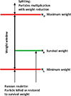 |
Fig. 7. Conceptual diagram illustrating weight window method. |
IM data is therefore used to compute the survival weight WS using equation (2).
 (2)
(2)
The maximum weight WU is then set to 2.0 ⋅ WS and WL is taken between 0.0 and WS (both excluded). Finally, the implicit capture variance reduction method is being developed in RayXpert® too. This method consists in preventing the capture processes, therefore the particles can continue their transports and have more chances to contribute to scores. All of these methods can be configured and specific biasing parameters can be set for any cell of the model allowing advanced and optimized biasing.
To illustrate the power of IM and variance reduction methods, an attenuation benchmark has been assessed. Figure 8 presents the geometry of this benchmark. The geometry is composed of 15 slices, 10 cm thick, made of water followed by 10 slices of same thickness made of concrete. At the end of the block, a 20 cm thick detector is placed. This detector is considered as the attractor for IM construction and is made of air. All material compositions are given in Appendix A (Tables A.1, A.2, A.3). A point photon source is placed at the position noted on Figure 8. It shoots 10 MeV photons along the  axis and the source intensity is set to 1.0 s−1.
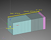 |
Fig. 8. Geometry of the attenuation benchmark. |
Figure 9 gives the total photon flux for each slice of the benchmark for 2 different configurations. The first configuration is an analog configuration: no biasing is used for this one. The second configuration uses the IM generated for this model and uses implicit capture, exponential transform and splitting biasing techniques. It is possible to observe from Figure 9 that as expected, photon flux decreases when going through slices for both configurations. Moreover, results are in very good agreement between the two configurations which is consistent with the use of biasing as it must not bias results but only improve Monte Carlo computation efficiency.
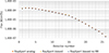 |
Fig. 9. Total photon flux for each slice (ordered from nearest to furthest from source) with 1 sigma uncertainties. |
To quantify the performances of a Monte Carlo simulation, the FOM (see Eq. (1)) is used as this indicator does not depend upon the number of primary particles simulated. The FOM of photon flux for each slice in each configuration of the attenuation benchmark is plotted on Figure 10. According to this figure, it seems that the FOM is in good agreement with the expected results. Indeed, for analog results, it is possible to see that the FOM decreases when going through slices. This is consistent as the benchmark represents an attenuation configuration. Therefore, fewer particles should reach slices far from the source resulting in a lower photon flux FOM for these slices. For the second configuration, a stable FOM is observed along the slices. This behavior could come from the fact that particles cannot be absorbed as implicit capture is used and cannot die as Russian roulette is disabled.
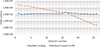 |
Fig. 10. Figure Of Merit for each slice (ordered from nearest to furthest from source). |
According to Figure 10, it is possible to see that the biased FOM is better than the analog one when getting closer to the IM attractor, up to a factor 50. Although the first slices show a decrease in efficiency (around a factor 10), it is possible to see that using IM and biasing seems to improve Monte Carlo computation efficiency around the attractor. Although these are preliminary results based on a simplistic benchmark, they nonetheless hold out the promise of potentially substantial gains in efficiency in suitable cases.
4.4. Geant4 coupling
Initially, RayXpert® physic are based on Geant4 physics. The physics of photons, neutrons, electrons, and positrons have been integrated into RayXpert®. In order to be able to simulate more types of particle and thus increase the field of application of RayXpert®, a bridge between RayXpert® transport feature and Geant4 physics is currently under development. This bridge will allow to make new particles available for the Monte Carlo simulation. Table 4 is a list of particles this bridge may be able to bring to RayXpert®. Thus, it will be possible to simulate with RayXpert® the radiation environment of other planets such as Mars, or the radiation environment of particle accelerators operating at high energies.
New particles handled in RayXpert® thanks to Geant4 bridge and available energy range of each particle.
4.5. Radiation Processing Module
In 2023, a new module for RayXpert® was released. This Radiation Processing Module (RPM) is designed to facilitate and bring new features related to the field of radiation processing and industrial sterilization, in ebeam and X-ray systems. It allows the user to directly set up a library of irradiation sites, defined once and for all the geometry and range of the irradiation configurations. It comes with a built-in library of conveyor systems, allowing the user to quickly create a model close to reality. Computation-wise, the RPM allows to consider of automated rotation of the irradiated product, double-side irradiation, multiple passes, throughput calculation, automated DUR (Dose Uniformity Ratio) the calculation and many more features well suited for the irradiation process. Figure 11 shows an overview of the RPM’s specific features.
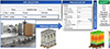 |
Fig. 11. Overview of the RPM’s specific features. |
4.6. Neutron-induced activation module
One of the most constraining phenomena when neutrons are simulated is neutron activation as neutrons produce radioactive nuclei for any energy range. Therefore, a new neutron-induced activation module is under development in RayXpert®. The Rigorous-Two-Step (R2S) methodology [37, 38] is used to simulate this phenomenon. The first step is to compute the neutron flux. Then, by using a state-of-the-art stiff differential equation solver, the inventory is accurately computed all over the geometry. Finally, decay rays are transported in the geometry through a Monte Carlo computation to compute the residual dose due to neutron-induced activation.
4.7. Update to the validation folder
As new features become available, RayXpert®’s validation folder will have to be updated to reflect the growing capabilities of the software. The projected addition to the validation folder includes a comparison of dose deposition for new particles (such as Braggs peak location, ion range in various materials, ...), reference activation scenario, and secondary particles creation rate for specific primary particles. These new validation files will be completed as needed to demonstrate and validate the new functionalities added in RayXpert®.
5. Conclusion
RayXpert® is a recent software launched just about a decade ago. Nevertheless, it is built on the shoulders of its sister software Fastrad®, which served as a stepping stone to provide numerous features in the very first release. The most important ones are the CAD geometry definition and STEP file import. Moreover, multithreaded 3D Monte Carlo computation for photons, electrons, and positrons was part of it from the beginning. Complex radioactive decay source definition was also among the first batch of features.
During the last decade, lots of new functionalities were introduced in RayXpert®. First, a TTB option was added, allowing huge efficiency improvement of Monte Carlo computation when simulating electrons. Then, a full mapping definition was added too. Cartesian, cylindrical, tetrahedral and surface mappings are available and results can be seen on an advanced post-processing viewer. Monte Carlo computation can be resumed through the usage of a resumption file. Flux-to-dose conversion coefficients are directly included allowing direct computation of relevant dosimetric estimator. A variance reduction biasing method based on strong assumptions is accessible. A built-in script engine is present and allows to manipulate RayXpert®’s objects and to automate repetitive tasks. A distributed version of RayXpert® is available. Neutron simulation is possible. Every particle result can be obtained with advanced convergence indicators. Thermal and molecular effects can be taken into account when simulating neutron transport too. Complex radioactive sources can be computed using a built-in Bateman solver. Pulse height scoring is also accessible allowing to replicate the response of a physical detector. A radiation processing module is also available and is designed to facilitate and bring new features related to the field of radiation processing and industrial sterilization. All these developments made RayXpert® a mature 3D Monte Carlo software at the cutting edge of technology.
Nevertheless, new features can still be implemented and improvements are being developed based in part on user feedback. Indeed, firstly an advanced biasing scheme is under development. This scheme has the ability to generate a model specific importance map for neutrons and photons. Then biasing techniques based on the usage of an IM are available. These techniques can be customized for any cell of the geometry. To demonstrate the capabilities of RayXpert® advanced biasing scheme, an attenuation benchmark was presented. Results obtained with biasing methods are in very good agreement with analog computation results. Using biasing technics has therefore enabled achieving an efficiency gain near a factor of 50. Hence, a biasing scheme under development seems to be able to improve Monte Carlo computation efficiency at least for this benchmark even if work is still needed to ensure faster results. A bridge between Geant4 and RayXpert® is under development allowing protons, ions and higher energy neutrons simulation. Finally, a neutron-induced activation module is under development and will be accessible in the future.
All these features make RayXpert® a suitable software for radiation protection studies as well as radiation processing mathematical modeling and the ongoing deployment of new features will further expand its range of applications.
Acknowledgments
We would like to thank the Geant4 project team for their contribution to science and computer science and for sharing their Geant4 Monte Carlo calculation code (Geant4 website: https://geant4.web.cern.ch/).
Funding
No external funding except for the radiation processing module (RPM) co-funded by IBA Group.
Conflicts of interest
The authors declare no conflict of interest.
Data availability statement
RayXpert® validation notes are available at the following address: https://www.rayxpert.com/validation-software/
Author contribution statement
All authors contributed to the development and implementation of the technical work described in this manuscript. A team of around 15 people working at TRAD – Tests & Radiations is dedicated to the development and validation of all the functionalities presented. Writing was coordinated by N. Dray, N. Mary, C. Dossat and J. Bourgoin. All authors proofread the final version of the paper.
Appendix A
Attenuation benchmark materials compositions
Water composition used for attenuation benchmark.
Concrete composition used for attenuation benchmark.
Air composition used for attenuation benchmark.
References
- N. Mary, RayXpert User Manual, Tech. Rep. TRAD/DL/DOS/RAYXPERT/CD/110412, TRAD - Tests & Radiations, 2024 [Google Scholar]
- P. Pourrouquet, J.-C. Thomas, P.-F. Peyrard, R. Ecoffet, G. Rolland, in FASTRAD 3.2: Radiation shielding tool with a new Monte Carlo module, 2011 IEEE Radiation Effects Data Worksho (2011) pp. 1–5 [Google Scholar]
- SNA+MC 2013 Annals of Nuclear Energy Special Issue, Ann. Nucl. Energy, 82, 1 (2015) [Google Scholar]
- MCNP Users Manual - Code Version 6.2, Tech. Rep. LA-UR-17-29981, LANL, 2017 [Google Scholar]
- E. Brun, F. Damian, C.M. Diop, E. Dumonteil, F.X. Hugot, C. Jouanne, Y.K. Lee, F. Malvagi, A. Mazzolo, O. Petit, J.C. Trama, T. Visonneau, A. Zoia, TRIPOLI-4®, CEA, EDF and AREVA reference Monte Carlo code, Ann. Nucl. Energy 82, 151 (2015) [CrossRef] [Google Scholar]
- W.A. Wieselquist, R.A. Lefebvre, SCALE 6.3.1 User Manual, Tech. Rep. ORNL/TM-SCALE-6.3.1, ORNL, UT-Battelle, LLC, Oak Ridge National Laboratory, Oak Ridge, TN, 2023 [Google Scholar]
- C. Geant4, Physics Reference Manual, Tech. rep., 2020 [Google Scholar]
- A. Ferrari, P.R. Sala, A. Fasso, J. Ranft, FLUKA : A multi-particle transport code, Manuel D’Utilisateur CERN–2005–010 INFN TC 05/11 SLAC–R–773, CERN, Genève (2011). [Google Scholar]
- S.J. Kemmerer, STEP, the grand experience, Tech. Rep. NIST SP 939, National Institute of Standards and Technology, Gaithersburg, MD, 1999 [Google Scholar]
- F.H. Attix, Introduction to Radiological Physics and Radiation Dosimetry, Physics Textbook (Wiley-VCH, Weinheim, 2004) [Google Scholar]
- C. Leroy, P.-G. Rancoita, Principles of Radiation Interaction in Matter and Detection, 2nd edn. (World Scientific, New Jersey, 2009) [CrossRef] [Google Scholar]
- G. Faure, Principles Of Isotope Geology (John Wiley & Sons Edition, New York, 1986) [Google Scholar]
- A.P. Dickin, Radiogenic Isotope Geology, 3rd edn. (Cambridge University Press, Cambridge, 2018) [CrossRef] [Google Scholar]
- R. Chandra, L. Dagum, D. Kohr, R. Menon, D. Maydan, J. McDonald, Parallel Programming in OpenMP (Morgan Kaufmann, Massachusetts, 2001) [Google Scholar]
- R. Emigh, Thick Target Bremsstrahlung Theory, Tech. Rep. LA-4097-MS, Los Alamos Scientific Laboratory, 1970 [Google Scholar]
- M.H. Mendenhall, R.A. Weller, A probability-conserving cross-section biasing mechanism for variance reduction in Monte Carlo particle transport calculations, Nuclear Instruments and Methods in Physics Research Section A: Accelerators, Spectrometers, Detectors and Associated Equipment, 667, 38 (2012) [Google Scholar]
- 5X Monte Carlo Team, MCNP-A General Monte Carlo N-Particle Transport Code: Version5 User’s Guide, Tech. Rep. LA-CP-03-0245, Los Alamos National Laboratory, 2005 [Google Scholar]
- ICRP Publication 74, Conversion coefficients for use in radiological protection against external radiation, Tech. Rep. Annals of ICRP 26(3/4), ICRP, 1996 [Google Scholar]
- Conversion Coefficients for Radiological Protection Quantities for External Radiation Exposures, Tech. Rep. ICRP Publication 116, ICRP, 2010 [Google Scholar]
- Conversion Coefficients for use in Radiological Protection Against External Radiation 2, Tech. Rep. ICRU Report 57, ICRU, 1998 [Google Scholar]
- J.M. Boone, A.E. Chavez, Comparison of X-ray cross sections for diagnostic and therapeutic medical physics, Med. Phys., 23, 1997 (1996) [CrossRef] [Google Scholar]
- ChaiScript - Easy to use scripting for C++., http://chaiscript.com/index.html [Google Scholar]
- W. Gropp, E. Lusk, A. Skjellum, Using MPI: Portable Parallel Programming with the Message-Passing Interface (Scientific and Engineering Computation, MIT Press, Cambridge, Mass, 1994) [Google Scholar]
- W. Gropp, E. Lusk, R. Thakur, Using MPI-2: Advanced Features of the Message-Passing Interface (The MIT Press, 1999) [CrossRef] [Google Scholar]
- V. F. Gaposhkin, Lacunary series and independant functions, Russ. Math. Surv. 21, 1 (1966) [CrossRef] [Google Scholar]
- M. B. Chadwick, M. Herman, P. Obložinský, M.E. Dunn, Y. Danon, A.C. Kahler, D.L. Smith, B. Pritychenko, G. Arbanas, R. Arcilla, R. Brewer, D. A. Brown, R. Capote, A.D. Carlson, Y.S. Cho, H. Derrien, K. Guber, G.M. Hale, S. Hoblit, S. Holloway, T.D. Johnson, T. Kawano, B.C. Kiedrowski, H. Kim, S. Kunieda, N.M. Larson, L. Leal, J.P. Lestone, R.C. Little, E.A. McCutchan, R.E. MacFarlane, M. MacInnes, C.M. Mattoon, R.D. McKnight, S.F. Mughabghab, G.P.A. Nobre, G. Palmiotti, A. Palumbo, M.T. Pigni, V.G. Pronyaev, R.O. Sayer, A.A. Sonzogni, N.C. Summers, P. Talou, I.J. Thompson, A. Trkov, R.L. Vogt, S.C. van der Marck, A. Wallner, M.C. White, D. Wiarda, P.G. Young, ENDF/B-VII.1, Nuclear data for science and technology: Cross sections, covariances, fission product yields and decay data, Nucl. Data Sheets, 112, 2887 (2011) [CrossRef] [Google Scholar]
- D. E. Cullen, PREPRO 2015 2015 ENDF/B Pre-processing Codes, Tech. Rep. IAEA-NDS-39, Rev. 16, IAEA, 2015 [Google Scholar]
- H. Bateman, Solution Of A System Of Differential Equations Occurring In The Theory Of Radioactive Transformations (1843) [Google Scholar]
- Thermal Scattering Law S(α, β): Measurement, Evaluation and Application - International Evaluation Co-operation Volume 42, Tech. Rep. NEA No. 7511, OECD/NEA, 2020 [Google Scholar]
- A. Milocco, A. Trkov, Quality Assessment of the IPPE Benchmark Experiments, Tech. Rep. IJS-DP-10217, IJS Internal Report, 2009 [Google Scholar]
- G. Manturov, Y. Rozhikhin, L. Trykov, Neutron and Photon Leakage Spectra from Cf-252 Source at Centers of Six Iron Spheres of Different Diameters, Tech. Rep. NEA/NSC/DOC/(95)03/VIII (ALARM-CF-FE-SHIELD-001), OECD-NEA, 2013 [Google Scholar]
- D.P. Gierga, K. J. Adams, Electron/Photon Verification Calculations Using MCNP4B, Tech. Rep. LA-13440, Los Alamos National Lab. (LANL), Los Alamos, NM (United States), 1999 [Google Scholar]
- J. C. Wagned, G. Radulescu, Specification for Phase VII Benchmark UO2 Fuel: Study of Spent Fuel Compositions for Long-term Disposal, Tech. rep., ORNL, USA, 2008 [Google Scholar]
- T.E. Booth, J.S. Hendricks, Importance estimation in forward Monte Carlo calculations, Nucl. Technol. – Fusion 5, 90 (1984) [CrossRef] [Google Scholar]
- M. Nowak, Accelerating Monte Carlo Particle Transport with Adaptively Generated Importance Maps, Ph.D. thesis, Université Paris-Saclay 2018 [Google Scholar]
- O. Petit, Y.-K. Lee, C.M. Diop, Variance reduction adjustment in Monte Carlo TRIPOLI-4® neutron gamma coupled calculations, Progr. Nucl. Sci. Technol., 4, 408 (2014) [CrossRef] [Google Scholar]
- N. Dray, Université Toulouse III – Paul Sabatier, Ph.D. thesis, 2022 [Google Scholar]
- N. Dray, E. Suraud, C. Dossat, N. Chatry, RayActive: An all-in-one R2S neutron induced activation analysis tool based on new intrinsic resolution methods, Nuclear Eng. Design 386, 111548 (2022) [CrossRef] [Google Scholar]
Cite this article as: Nicolas Dray, Nicolas Mary, Cédric Dossat, Jefferson Bourgoin, Nathalie Chatry. An overview of last decade’s developments in RayXpert®, a 3D Monte Carlo code, EPJ Nuclear Sci. Technol. 10, 10 (2024)
All Tables
New particles handled in RayXpert® thanks to Geant4 bridge and available energy range of each particle.
All Figures
|
Fig. 1. Screenshot of the RayXpert® GUI with a STEP imported geometry example. |
| In the text | |
|
Fig. 2. Photon flux results obtained on a Cartesian mapping with RayXpert®. |
| In the text | |
|
Fig. 3. Example of tetrahedral mapping generated with RayXpert®. |
| In the text | |
|
Fig. 4. Time decay solver results obtained with RayXpert® for the lump of 238U. |
| In the text | |
|
Fig. 5. Pulse height score for 192Ir spectrum with (orange) and without (blue) GEB. |
| In the text | |
|
Fig. 6. Example of the photon importance map generated with RayXpert® between 32 keV and 1.0 MeV for the geometry presented in Figure 2. |
| In the text | |
|
Fig. 7. Conceptual diagram illustrating weight window method. |
| In the text | |
|
Fig. 8. Geometry of the attenuation benchmark. |
| In the text | |
|
Fig. 9. Total photon flux for each slice (ordered from nearest to furthest from source) with 1 sigma uncertainties. |
| In the text | |
|
Fig. 10. Figure Of Merit for each slice (ordered from nearest to furthest from source). |
| In the text | |
|
Fig. 11. Overview of the RPM’s specific features. |
| In the text | |
Current usage metrics show cumulative count of Article Views (full-text article views including HTML views, PDF and ePub downloads, according to the available data) and Abstracts Views on Vision4Press platform.
Data correspond to usage on the plateform after 2015. The current usage metrics is available 48-96 hours after online publication and is updated daily on week days.
Initial download of the metrics may take a while.