| Issue |
EPJ Nuclear Sci. Technol.
Volume 8, 2022
|
|
|---|---|---|
| Article Number | 6 | |
| Number of page(s) | 14 | |
| DOI | https://doi.org/10.1051/epjn/2022001 | |
| Published online | 20 May 2022 | |
https://doi.org/10.1051/epjn/2022001
Regular Article
Modelling of radioactive dust for dose calculations with stochastic geometries
Université Paris-Saclay, CEA, Service d'Études des Réacteurs et de Mathématiques Appliquées, 91191 Gif-sur-Yvette, France
* e-mail: This email address is being protected from spambots. You need JavaScript enabled to view it.
Received:
30
September
2021
Received in final form:
2
December
2021
Accepted:
1
February
2022
Published online: 20 May 2022
Abstract
Stochastic geometries in Monte-Carlo simulations enable to simulate complex configurations such as the repartition of possible radioactive dust in a glove box. This paper compares several dust models that represent more or less explicitly the heterogeneous repartition of dust speckles in space. Indeed, assessing the contribution of dust to the dose received by the hands of an operator is a key problem for glove boxes. Results show that homogeneous models generally overestimate the dose, which is correct for radioprotection studies, but that dust aggregates produce doses that are much smaller than those obtained by homogenising dust. These heterogeneous models can also help estimating deposited dust quantities from dose measurements inside the glove box, whereas an homogenous model would grossly underestimate dust quantity.
© A. Bonin et al., Published by EDP Sciences, 2022
 This is an Open Access article distributed under the terms of the Creative Commons Attribution License (https://creativecommons.org/licenses/by/4.0), which permits unrestricted use, distribution, and reproduction in any medium, provided the original work is properly cited.
1 Introduction
Glove boxes are used in research laboratories and in the nuclear industry to isolate an operator from radioactive material. Some operations carried out in glove boxes can lead to the formation of radioactive dust, which remains suspended in the air before settling. If this dust is present in large quantities, it can contribute significantly to the dose received by the operator of the glove box. Besides, even if present in small quantities, dust might accumulate repeatedly in the same place, e.g. in the lower corners of the glove box or near the gloves, and also lead to significant doses. For this reason, glove boxes are regularly cleaned out of dust.
Radiation protection calculations for glove boxes can take into account the presence of dust. Because of the capabilities of simulation codes, so-called homogeneous models are generally used. A homogeneous dust model replaces volumes of air in certain areas of interest containing dust in the glove box with volumes of radioactive material of extremely low density. This fictive density is calculated from the quantity of air and radioactive material included in the volume. The model is homogeneous because this density is constant in the volume to be analysed.
Recent advances in stochastic geometry [1] in Monte-Carlo simulation models such as TRIPOLI-4® [2] make it possible to consider a stochastic modelling of dust accumulations, by generating and setting in space for example a very large number of spheres of variable radius representing the position of the dust grains. Mixed strategies combining homogeneous modelling and dust grains can also be considered.
This paper presents new models for dust simulation in a glove box. The calculated doses are compared in different configurations, in order to determine whether homogeneous models systematically lead to overestimating the received doses, which would be a good property for radiation protection calculations, and in which configurations a more refined modelling of the dust geometry is useful.
2 State of the art
Radiation protection calculations are generally based on the following principle: determination of particle sources (intensity, spectrum), transport of these particles in geometries representing the geometric configuration of the environment, and finally dose calculation at several points of interest.
The particle transport simulation models used for dose calculations are based on the resolution of the Boltzmann particle transport equation. Stochastic geometries have been used in particle transport simulations with Monte Carlo models over the last few decades [1–3]. These methods have been used in several criticality applications, such as pebble-bed reactors [4,5] or waste storage container [6] for example. To our knowledge, they have not yet been used for radiation protection applications.
One of the Monte Carlo transport codes commonly used is TRIPOLI-4® developed at CEA. A new tool, recently developed at CEA, is dedicated to the generation of stochastic geometries. A coupling of this generator with TRIPOLI-4® makes possible to perform transport in random geometries in the frame of the so-called quenched disorder approach [7–9]. The scheme is the following: a large number of random geometries is generated, then we solve the Boltzmann equation for each geometrical configuration and calculate some observables of interest (such as flux, reactions rates, neutron multiplication factor etc.) and finally we compute the ensemble-averaged quantities for the target observables. This method allows to compare the results obtained for criticality problems between the stochastic geometries and a regular network of fissile debris in water and to show that taking into account the stochastic media has an impact on the neutron multiplication factor [10]. Note that dust computations do not require to estimate a mean behaviour as the dust geometry is static, but unknown. Thus it is important to assess how far the estimated doses vary with respect to the geometry randomness.
A critical parameter in the study of particle transport in a stochastic medium is the mean chord length Λn [11] characterising each material noted n composing the medium. It is defined by the average length of the path that a particle can follow in a straight line through this material n. Since the medium is random, the chord lengths vary around this average value.
The comparison between the average chord length in material n and the average free path of the particles in this material shows whether the medium can be homogenised or not:
if ΛnΣt,n « 1, Σt,n being the total effective cross-section in material n, this means that during a typical path (mean free path) the particle will see a large number of chunks of material n. If this assertion is true for each material n composing the medium, the exact location of these chunks does not matter, only their average number: this is the “atomic mix limit” regime [12], in which the stochastic medium can be modelled homogeneously (by defining an homogenised material whose physical properties, such as cross sections, are computed by averaging the physical properties of each material).
conversely, if there is at least one material n such that ΛnΣt,n ≫ 1, the particle may during a typical displacement (mean free path) encounter only one material. In this case, the stochastic medium must be modelled more finely, especially if the material chunks are spatially unevenly distributed.
The homogenisation of a medium is in many radiation protection problems a good compromise between the accuracy of the results and the calculation time. However, in some cases, it is necessary to model the stochastic geometry in detail in order to estimate more accurately the equivalent dose rate, for example, or other quantities of interest.
The integral form of the transport equation is written for the collision density ψ, that is the number of particles arriving with speed E and colliding in r [13]: (1)where E: speed variable grouping the energy E and the direction of the trajectory of the particle
  , ΣT (r, E) : total macroscopic cross-section (cm−1), ΣS (r, E′ → E): differential scattering cross section shifting the speed from E′ to E (cm−1 MeV−1 st−1), R: distance (cm) between the position of the particle before the collision r′ and its position at the time of the collision r, the vectors r′ and r verify
  , S (r, E): particle source density (particles cm−3 s−1 MeV−1 st−1), ψ (r, E): collision density of particles entering a collision at r with velocity E (particles cm−3 s−1 MeV−1 st−1), ψ (r, E) = ΣT (r, E) φ (r, E), φ (r, E) dE: particle flux at position r and with velocity between E and E + dE (particles cm−2 s−1).
In the above equation (1) τ is the optical distance corresponding to the geometric distance R between two collisions located in r′ and r: (2)
(2)
When a heterogeneous medium is modelled with a homogeneous material, the total macroscopic cross section does not depend on the position of the particle in space but only on its energy. The macroscopic cross section of diffusion also depends only on the energy of the particle. The average distance between collisions is given by the mean free path: (3)
(3)
This paper considers the problem of random dust in a glove box, thus a very small quantity of material in a large volume of air. If the material is homogenized, the equivalent densities will be very low.
The probabilities of diffusion, that depend on ΣS, and the probabilities of absorption, that depend on ΣT, do not vary spatially and are quite small because of the low density of the homogenized medium.
Besides, if a stochastic model is used for the medium, the probabilities of diffusion and absorption depend not only on the energy but also on the position and direction of the particle. The collisions are distributed in a disparate way and can be concentrated in certain locations, where materials have a higher density.
3 Simulated configuration and dust modelling
3.1 Typical glove box and radioactive material
The simulated glove box is supposed to contain a conic jar full of typical (U,Pu) oxide powder, a pellet basket and a pressing table. This glove box is inspired from pelletizing workplace in a uranium oxide or mixed-oxide fuel fabrication facility [14,15]. The jar is located above the press table where pellets are made before being transferred into the pellet basket.
3.1.1 Geometrical model
The glove box is made of a stainless steel envelope at its backside and of Kyowa Glass shield at its frontside, where an operator can stand.
The glove box in this model contains three main radioactive sources:
a conic jar made of stainless steel and surrounded by a radiation shield, containing tens of kilograms of MOX powder;
a press table with tens of grams of MOX pellets upon it;
a pellet basket, containing a few kilograms of pellets.
Another radioactive source is the dust from the oxide mixture powder that may have spread into the glove box, settled on the Kyowa Glass protection and accumulated in certain areas of the glove box as well as in the lower corners of the glove box (see Fig. 1). The modelling of this dust is the subject of this paper.
The dust grains can be UO2, PuO2 or MOX grains. The two important parameters for modelling oxide mixture dust are the radii of the dust grains and their spatial distribution. The diameter of UO2 and PuO2 grains in several fuel fabrication facilities has been measured and is reported in various publications [16–22]. The AMAD (Activity Median Aerodynamic Diameter) is estimated between 2 and 10 micrometers depending on the area of the installation. In addition, the dust grains can agglomerate and form aggregates [21], which can reach a size of more than 100 micrometers [23].
In the dust model proposed here, the grain radius varies between 50 and 1000 micrometers. Dust grains of radius lower than 50 micrometers are not considered in this paper because this size of geometrical object is at the boundary of what the simulation code can handle safely. Actually, the dust grains simulated in this paper represent compact symmetrical aggregates as observed in [23]. Besides, an explicit model for more general aggregates is proposed at the end of the paper.
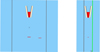 |
Fig. 1 Visualisation of sections of the glove box model obtained with TRIPOLI-4® viewer: (y,z) plane on the left, and (x,z) plane on the right. The red cone represents the mixed oxide in the jar, the red rectangle in the centre the pressing table and the cross at the bottom right the corner full of dust, just behind the Kyowa Glass (in green in the figure). |
3.1.2 Dust deposition sites
To choose the location of the dust grains, a few assumptions are made: firstly, it is assumed that the scenario in which an operator may intervene in the glove box is a maintenance operation, and therefore all machines have been stopped long enough for all the dust to have settled on the glove box surfaces. All dust is therefore assumed to have deposited to the walls and floor of the glove box and its arrangement does not change over time. Thus, airborne dust is not taken into account. The most likely points of accumulation are the surface of the Kyowa Glass protection and the bottom of the glove box. In addition, it is assumed that due to the difficulty of routine cleaning, dust grains mainly accumulate in the lower corners of the box. With the homogeneous model, dust deposited on the Kyowa Glass is simulated by a thin parallelepipedic layer on the Kyowa Glass inside the glove box and dust accumulated in the two lower corners of the glove box is simulated by two 5 cm cubes. In this paper we are interested in the two lower corners next to the Kyowa Glass protection.
3.1.3 Composition
The fuel is the one used in [24], a typical Mixed Oxide (MOX), whose composition (cf. Tab. 1) is comparable to the typical ones used in Light Water Reactors.
Heavy metal composition of a typical mixed oxide.
3.1.4 Calculation of the equivalent dose rate
There are three main radiation sources coming from the dust grains of oxide mixture: neutron rays emitted from spontaneous fission and from (α,n) reactions, primary gamma-rays emitted from actinides and secondary gamma rays emitted by the radioactive capture of neutrons in matter.
The primary neutron and gamma sources, emitted directly from the oxide mixture, are computed by the DARWIN evolution code [25] for a cooling time of 2 years. The nuclear data and the decay chains used in the computation come from the JEFF-3.1 Nuclear Data Library [26]. The total intensity of neutron source, including neutrons from spontaneous fissions and neutrons from reactions (α,n) on the oxygen atoms in the mixture, is calculated by DARWIN code. The neutron spectrum is distributed according to a Watt spectrum with coefficients 1.0352 MeV−1 and 2.8420 MeV−1, taken from the American evaluation ENDF/B-V [27] and that corresponds to fissions due to thermal neutrons of Pu. The gamma spectrum is calculated with DARWIN on an energy grid with 220 groups.
The Ambient dose equivalent H*(10) is the operational quantity used to monitor external exposure to penetrating radiation in an area [28,29]. Ambient dose equivalent H*(10) (μSv/h) due to neutron and photon radiations emitted by the (U,Pu)O2 mixture is computed by the TRIPOLI-4® code. The dose due to neutrons and gamma coming from (n,γ) reactions taking place in the various radiation shields is also computed. Moreover, the dose due to gamma emitted directly by the (U,Pu)O2 mixture, is computed in 220 energy groups.
The total dose due to neutrons and gamma rays emitted by the oxide mixture constituting the deposited dust grains is thus calculated first from a homogeneous dust model − described in Section 3.2 – and then from several new refined heterogeneous models using randomly distributed spherical inclusions − described in Sections 3.3, 3.4 and 3.5.
3.2 Homogeneous model
The simplest way to model a disordered medium is to homogenize it. The goal is to have a configuration with the same macroscopic properties as the real medium in average, but with a much simpler geometry. The radioactive material is diluted within a chosen volume that is as close as possible to the volume actually occupied by the radioactive material. Instead of considering a disordered geometric arrangement of dense and compact dust grains, radioactive dust will be simulated as a homogeneous source, with a simple geometric shape and with a lower density. The macroscopic cross-sectional efficiencies of the homogenized medium are obtained by averaging the cross-sectional efficiencies of each material weighted by the respective volume ratio of each material.
With the homogeneous model, the geometric shape of the source is fixed, only its mass varies, by changing the density of the emission volumes to simulate different dust densities.
The limit of the model is the alteration of the properties of the medium at the microscopic scale. The mixture configurations in which it is reasonable to use homogenization of the properties while maintaining unaltered transport properties such as cross sections and sources, require a mean free path greater than the maximal mean chord length characterizing the medium (atomic mixing model). If this assumption is not filled, the chord length distribution associated with the model of stochastic geometries has to be taken into account. For some particles, such as gamma photons, the mean free path in metals can be very small. In addition, dust grains have a very small mean diameter [21,23], ranging from micrometers to hundreds of micrometers, dispersed in an air matrix.
3.3 Spherical inclusions created by random sequential addition
3.3.1 Identical spherical inclusions
A very large number of identical spherical sources are dispersed in an air matrix. The basic Monte Carlo method for generating a stochastic distribution of non-overlapping spheres is the random sequential addition method [30,31]. The spheres are created in the same control volume as the one used for the simulation of the homogeneous model, which will allow to compare the two models.
In the case of spherical inclusions with identical radii, the number N of spheres to be generated is computed as follows:
where ξ is the inclusion occupancy rate or packing fraction, i.e. the ratio between the volume occupied by the spheres and the control volume V (see Sect. 2.2.4), in which the inclusions are generated.
In the cubic control volume the spheres must not intersect the walls of the box, the random sampling of the first centre of the inclusion is calculated by generating, according to a uniform distribution, three random numbers in the range [–L/2+R; L/2–R], where L denotes the size of the box and R denotes the radius of the spheres.
The algorithm used in this study is an improvement of the random sequential addition method: it consists in creating within the control volume a spatial cartesian mesh whose base cell has a dimension greater than or equal to the diameter of the spheres [12]. The spatial mesh reduces the computation time to test if spheres overlap: when a new sphere is introduced in the control volume, the mesh enables to get the closest spheres that are the one contained in adjacent cells.
With this type of random geometries, there are three free parameters: the occupancy rate (packing fraction) ξ, the material density in each sphere and the radius of the spheres. Two strategies can be considered to cover different cases:
increase the packing fraction ξ, which modifies the emissivity of the source depending directly on the mass of the radioactive material and therefore on the number of spheres, without modifying the properties of each sphere;
simultaneously modify the radius of the spheres and ξ, the material density of each sphere being constant, which modifies the transport properties while keeping the emissivity of the source constant.
3.3.2 Spherical inclusions with random radii
While spherical inclusions with identical radii are a simple approach to modelling at the microscopic scale, spherical inclusions with random radii allow a better simulation of reality. For the purpose of illustration, an example of geometry obtained with the method of spherical inclusions with random radii is shown in Figure 2.
For the generation of a geometry with spherical inclusions of random radii [12], the values of the radius of the spheres must be randomly sampled from a given probability law, before the inclusions are generated. Specifically, two PDFs have been used for this purpose: a uniform distribution and a log-normal distribution with parameters μ = 2.4 μm and σ = 0.84. The spheres are added progressively until a higher occupancy rate than the one chosen is reached. At this point, the radius of the last generated sphere is modified in order to obtain the exact occupancy rate ξ. Then the spheres are ordered by descending radii. The centre of a sphere is uniformly sampled such as the sphere does not overlap the boundaries. A list of the mesh cells that the sphere intersects is determined. A check is performed to verify whether the sphere overlaps any of the spheres already contained in these mesh cells.
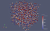 |
Fig. 2 Simulation of the corner of the glove box with spherical inclusions. |
3.4 Spherical inclusions with “cannonball” distribution
An original algorithm for spherical inclusions is proposed here. It consists in the construction of a stack of non-overlapping spheres as dense as possible using the so-called “cannonball” distribution. A box is thus filled by a face-centred cubic lattice. Then, to give shape to the geometry, a rejection test is applied, according to different types of geometrical shapes (sphere octant, hyperbole, cubic). The last step consists in applying a Russian roulette technique on the non-rejected spheres, in order to obtain the total mass or the desired number of spheres.
The FCC − face-centred cubic − lattice is formed inside a cube l ∙ l ∙ l, using trigonometric formulas that link the position of the centre of a sphere to the position of the centre of its neighbouring spheres. In 1D, the distance between two neighbouring spheres is equal to the diameter of the spheres. In 2D, many rows are superimposed with a horizontal pitch of value 2r ⋅ cos (π/3), while the vertical pitch between two successive rows is equal to 2r ⋅ sin (π/6). Finally, the same mechanism is applied for the third direction as for the second: each plane is spaced from the other planes of 2r ⋅ cos (π/3) with respect to the others, and each plane has a vertical and horizontal pitch with respect to its neighbour. To avoid overlapping of the spheres through the walls of the cube, this procedure can be carried out by excluding all spheres whose centre is at a distance from the wall less than its radius.
Once the lattice of spheres has been generated, in order to give the geometry the desired shape, a mathematical expression of a geometric form is chosen to reject all the spheres contained, or not contained, inside it, as mentioned above.
The simplest rejection test is carried out using a sphere of radius r = l centred in a corner of the cube. In this way, it is possible to obtain a shape that is the whole cube minus one eighth of a sphere.
The analytical expression that the centre of the spheres must satisfy in order not to be excluded is therefore: where (xc, yc, zc) are the coordinates of the centre of a sphere.
The volume occupied by these spheres is  , giving a sphere occupancy rate of about 0.7. Such an occupancy rate of 0.7 is high and will lead to a number of spheres that could (depending on the radius with respect to the size of the control volume) possibly be too large for the dataset to be processed by TRIPOLI-4® in a reasonable time.
A Russian roulette technique is applied to randomly reject unnecessary spheres, keeping the shape of the geometry. To apply the Russian roulette, a desired mass m is chosen. In the case of spherical inclusions of mono-dispersed radius, this leads directly to the number of spheres. The number of spheres necessary to obtain this mass is thus calculated:
If this number is less than the number of spheres already generated, we introduce the probability of rejection PRussian, which can be calculated either as  or
or  , where Ntot and mtot are respectively the number of inclusions and the total mass of the spheres before rejection. Then, a random variable ζ is uniformly generated between 0 and 1 for each sphere, and all spheres that do not satisfy ζ < PRussian are rejected and stored in a second table.
Once the rejection loop is completed, there is a final check on the number of remaining spheres: if this number is greater than the desired number, the rejection process is repeated by randomly rejecting the unwanted spheres with the same system. If this number is less than the desired number, the remaining centres are randomly selected from the table of previously rejected spheres.
This algorithm, even if the stochastic nature of the geometry is partially lost due to the creation of the FCC array, gives the possibility to realistically arrange the dust, and to have a much higher occupancy rate than with the RSA (Random Sequential Addition) method.
The geometry closest to the actual dust geometry is obtained by using a surface defined by three hyperbolic cylinders, instead of the spherical surface previously proposed for the first rejection test.
The analytic expression of the volume of dust is defined as follows:


The parameters of the three hyperbolic paraboloids are chosen so that dust accumulates more horizontally due to gravity. This geometry is shown in Figure 3.
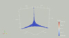 |
Fig. 3 Representation of the geometry obtained from the intersection of the original cube with 3 hyberbolic cylinders for 5 g of spherical inclusions with a radius of 0.025 cm. |
3.5 Dust aggregates
In a glove box, dust grains often accumulate at the same place to form aggregates.
Here two models of a dust aggregate are compared. The first one consists in creating an analytical distribution of spheres inside a larger sphere [32,33], itself randomly placed in the cube using the RSA method. The analytical distribution of spheres is a dense stack of twelve spheres. The occupancy rate within the large sphere is at most 49% with this type of arrangement of spheres (cf. Fig. 4). However, it was necessary to add a small extra space between the spheres because of the geometrical accuracy of the Monte Carlo transport code TRIPOLI-4®, which leads to an occupancy rate of 42%.
The second modelling consists in homogenizing in the volume of the large sphere the twelve small spheres, as mentioned above.
Using the TRIPOLI-4® code, it is thus possible to simulate the two configurations: the large sphere containing the densest possible set of twelve small spheres, and the same large sphere in which the small spheres have been homogenized in volume, considering the appropriate void fraction.
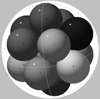 |
Fig. 4 Drawing of the dense 12 spheres hexagonal close packing inside a bigger sphere (source: https://en.wikipedia.org/wiki/Sphere_packing_in_a_sphere). |
4 Simulation strategies
The main problem in Monte Carlo simulation of a dispersed source, such as spherical MOX inclusions, is the sampling of particle emission sites in sources. Since the simulation of particle transport is performed by a random Markov walk, the starting point of the walk is randomly sampled within the source volume. More precisely, the declaration of a source consists in giving the code the coordinates of a mesh, parallelepiped in this study, and information to indicate which volumes within this mesh are emitters. In this way, the code randomly samples a given number of points within the mesh, and if that point falls within a fissile volume, another random sampling begins to select the energy and direction of the particle. Thus, the starting point of the random walk is chosen by a rejection process.
In the case of the homogenized model studied here, the homogenized source is of parallelepiped shape, so the rejection efficiency, which is equal to the ratio between the volume of the parallelepiped used as a control volume and the volume of the source itself is equal to 1. (4)
(4)
In contrast, with the spherical inclusion source model, the fissile volumes are dispersed in the air matrix, and the fraction of the volume occupied by the source may be less than 1% of the total volume. In order to have a good source convergence it is necessary to have a huge number of random samplings to obtain a good accuracy, according to the derivation of the Monte Carlo Central Limit Theorem:
In this equation  represents the relative error with respect to the exact result μ weighted on the sample average
  and
and  represents the PRSD (Percentage Relative Standard Deviation), where σ2 is the variance and N the number of random samplings.
In addition, the probability of success of random sampling is very low, so there can be huge fluctuations in the average value of the sample. The solution is to improve the efficiency of the rejection by taking a single cubic cell around each emitting sphere instead of a single parallelepiped encompassing all sources and coinciding with the control volume used to generate the spherical inclusions.
In this case, the efficiency is significantly improved and it becomes:
Indeed, this efficiency is higher than that obtained by using the same control volume for spherical inclusion generation and source sampling, which is worth at most ξMAX,RSA=0.38.
The approach using a parallelepiped cell for each emission volume of the source increases slightly the simulation time and is only used when it is necessary. For example, in the case of spherical inclusions built using a FCC lattice, the occupancy rate is high and the control volume is then used as the reject volume. In the case of special source geometries such as hyperboles, the reject volume is adapted as much as possible to the geometry by using several parallelepipeds.
Regarding the simulation of the aggregates, the packing fraction within each large sphere is quite high (about 42.4%), so using the same method as for stochastic spherical inclusions, according to equation (3), it is possible to have a rejection efficiency equal to
where ξ′ is the packing fraction inside the large sphere. So, in the case of a dense packing of twelve spheres inside a sphere, the rejection efficiency can be written as:
These optimization techniques become very important when the number of spheres becomes very large.
It is also possible to speed up the simulation by creating a connectivity map specific to the geometry being studied. To do this, a mesh is first created inside the volume containing the stochastic inclusions, in order to divide this volume into several volumes containing only a small number of inclusions. The connectivity map itself is the list of volumes present in the geometry coupled to their neighbours. Such a map allows to speed up particle tracking, especially for configurations with a large number of spheres (typically, the impact of the connectivity map is clearly visible for configurations with more than 105 spheres). This mesh is also useful to define more quickly the interfaces between the different volumes present in the glovebox and the numerous spherical inclusions.
5 Results
All the results are equivalent dose rates computed with the ambient dose equivalent H*(10) as defined in Section 3.1, in μSv/h. The objective is to estimate the contribution of the dust inside the glove box to the extremity dose, for example to the hands of an operator working in maintenance. The dust is placed in the two lower cubic corners of 5 cm side, juxtaposed to the Kyowa Glass shield. The dose is calculated at a point sufficiently close to the dust, 15 cm from a lower corner (cf. Fig. 5), and also at a point right over the pressing table, more than 1.30 meters above the dust (cf. Fig. 6).
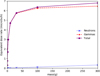 |
Fig. 5 Homogeneous model, Corner source with parametrical variation of the density, results at 15 cm from the source. |
 |
Fig. 6 Homogeneous model, Corner source with parametrical variation of the density, results right over the press. |
5.1 Homogeneous model
The dust is homogenized by considering that it is “diluted” in the air of each 5 cm cubic corner. The amount of dust deposited in a corner ranges from 0.1 to 300 grams by varying the fictitious density of homogenized dust diluted in the corner from 0.0008 g/cm3 to 2.4 g/cm3. The transport properties change a lot, because particle diffusion is influenced by the macroscopic cross-sections of the medium, which depend directly on the number of nuclei in the particle path (quantity directly correlated to the density).
The calculations with TRIPOLI-4® for the neutron dose are made using 20,000 batches of 3000 particles each and at least 300,000 batches of 5000 particles for the gamma dose. The standard deviation for neutron calculations does not vary much from case to case, while the standard deviation for gamma calculations varies a lot. Indeed for gammas the convergence speed decreases with increasing density, because the amount of gamma particles that can escape from the source decreases as the density increases. As the standard deviation are inferior to 0.24% for neutron calculations and inferior to 0.57% for gamma calculations with the homogeneous model, they are not represented in the following figures.
A saturation effect is observed for the dose due to gamma rays (cf. Figs. 5 and 6). The cause of this saturation is the increase in the effective absorption cross section of the source itself and thus the decrease in the mean free path of the gamma rays, which makes difficult or even impossible for these particles to escape from the environment. Gamma rays are very well stopped by metals, whereas neutrons have a much longer mean free path.
The equivalent dose rate due to neutrons is considerably lower than the equivalent dose rate due to gamma, therefore in the following only the equivalent dose rate due to gamma will be presented.
5.2 Spherical inclusions of same radius
The source consists of a set of small spheres placed randomly thanks to the algorithm described previously (Sect. 3.3) instead of a single, larger homogeneous volume.
5.2.1 Variation of the radii of the spherical dust grains
The dust deposited in a corner of the glove box is modelled using spherical inclusions created using RSA techniques, presented in Section 3.3. The use of the RSA method allows us to act on the emission of small spherical sources without modifying their inner density or mass. Only the radius of the spherical sources varies from 1 mm to 100 microns (cf. Tab. 2).
The total mass of the sources is fixed at 1 g, which is equivalent to a packing fraction set the value ξ = 0.00121. In this experiment, simulations with quite a small source diameter are not trivial to perform. Indeed, to simulate one gram of dust using spheres of diameter d = 100 μm, the number of source volumes in each corner is almost 300,000. This naturally leads to a very long calculation time (more than one hour on a state of the art workstation), even after using the acceleration methods described in Section 4.
A decrease in the radius of the emitting sphere leads to a greater leakage of gamma particles from this sphere and a consequent increase in the overall dose rate. In a convex geometry containing spherical inclusions of radius r in a matrix, the expression of the mean chord length in the matrix is written [34]:
Since the radius of the spheres is directly proportional to the average chord length of the geometry, decreasing the radius of each emitting sphere, while keeping the density and total mass of the source constant, means getting closer to the atomic mix. The results with very small spheres are close to those obtained using the homogeneous model (cf. Fig. 7).
The curve of the equivalent dose rate versus the radius of the source spheres is almost exponential. Indeed, the attenuation of the radiation flux inside an absorbing medium follows an exponential law. The average chord length is defined as the average length of absorbent material that a particle travelling in straight line encounters during its path. It is intuitive that a decrease in the radius of the spheres leads to a decrease in the average thickness of the absorbing medium through which the particle passes and simultaneously to an increase in the leakage of particles out of the source spheres, therefore an increase in the dose.
RSA spherical inclusion method, equivalent dose rate (EDR) calculated for different values of the radius of the source spheres.
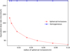 |
Fig. 7 RSA spherical inclusion method, Gamma simulations with different values of the sphere radii with a constant mass of 1g for each corner and constant density of 6.6 g/cm3 (relative standard deviation inferior to 1%, given in Tab. 2, are not presented on the figure). |
5.2.2 Variation of the total mass of dust grains
The radius of the spheres is set at R = 0.05 cm, the density at 6.6 g/cm3 and the total mass of dust varies from 1 g to 100 g, corresponding to a variation in the packing fraction from 0.00121 to 0.121. The density of 6.6 g/cm3 is the one of raw fuel pellets that have not been sintered yet, and thus is lower than the usual density of around 10 g/cm3. As the packing fraction increases, the dose curve approaches the homogeneous model (cf. Fig. 8). From a dust quantity of more than 100 g a saturation effect appears on the dose curve.
These two figures lead to the conclusion that, on the one hand, at constant occupancy rate, the larger the dust radius, the farther the model differs from the homogeneous model, and, on the other hand, at constant radius, the smaller the amount of dust, the farther the model differs from the homogeneous model.
As for the equivalent dose rate due to neutrons, the stochastic geometry model with spherical inclusions provides results very close to those obtained with the homogeneous model (cf. Fig. 9). The difference between the neutron equivalent dose rate of the dust simulated using any stochastic geometry and the homogenized dust is less than the standard deviation of the TRIPOLI-4® results. Simulations are performed with 200 batches of 3000 particles each, for an accuracy of PRSD ∼2.5%. The gammas have a mean free path comparable to the characteristic dimensions of the simulated medium, but the neutrons have a much longer mean free path and the homogeneous model is sufficient.
As indicated above, the source is a set of very small spheres instead of a single, larger homogeneous volume. As this source geometry is obtained with a stochastic algorithm (cf. Sect. 3.3). It is important to check how the different spatial arrangements of the spheres influence the results. To investigate the effects of stochasticity on the evaluation of equivalent dose rate, 100 geometries have been simulated with different random seeds to analyse qualitatively the distribution of dose rates. The number is too small to estimate complex distributions. However, histograms are provided, as well as empirical standard deviation. The control volume in which the spherical inclusions are generated is the cubic corner, in which homogenisation is applied in the case of the homogeneous model. The packing fraction ξ, the radius and the material density of the spheres are constant.
The simulated mass in the test volume is equal to 1 g, which corresponds to a fraction of ξ = 0.00121 and 287 spheres with a radius of half a millimetre. The equivalent dose rate (expressed in μSv/h) due to gammas are presented in Figure 10.
Each simulation uses 1000 batches of 5000 particles, for a precision of less than 1%. The equivalent dose rate varies very little with respect to the geometry randomness. The mean of the 100 realizations is of 47.7 μSv/h and the empirical standard deviation of 0.74 μSv/h, which corresponds to 1.5% of the response.
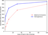 |
Fig. 8 Spherical inclusion model, Gamma simulation with spheres of constant radius of 0.05 cm, constant density of 6.6 g/cm3 and variable packing fraction (PRSD are inferior to 1%). |
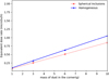 |
Fig. 9 Spherical inclusion model, neutron simulation with spheres with a fixed constant radius of 0.05 cm and a constant density of 6.6 g/cm3 with variable packing fraction (PRSD are inferior to 1%). |
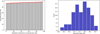 |
Fig. 10 100 realizations of spherical inclusions with R = 0.05 cm, ξ = 0.00121 and ρMOX = 6.6 g/cm3 (left: realizations ordered by dose rate, with 2-sigma error bars in red and right: histogram). |
5.3 Inclusions with random radii
When it comes to inclusions with random radii, some parameters that were constant with the packing fraction in the simulations with identical inclusions becomes case-dependent. It has been shown that the mean chord length of the distribution through spheres with random radii is inversely proportional to the second-order moment of the radius [12,35], which in this particular case may change according to the values of the radius of randomly sampled spheres. For this reason, at a fixed packing fraction and fixed mass, the results of the simulation vary more according to sampling.
In this simulation, the values of the radius are homogeneously sampled between 1 mm and 10 micrometers, according to a uniform probability density function. Identical inclusions have all a 1 mm radius. With spherical inclusions of random radii the dispersion between the results of the 100 realizations is much greater than that obtained with identical spherical inclusions (cf. Figs. 10 and 11). The distribution is not symmetrical, and has an empirical standard deviation of 5.5 μSv/h for a mean of 26 μSv/h, which corresponds to more than 20% of the response. The actual distribution of the response when the geometry varies due to randomness could be investigated with a much larger number of simulations. However, the simulated dose can vary from 10 to 35 μSv/h depending on the spatial repartition of dust grains in the control volume, which suggests that spatial dust repartition might have a significant effect on dose for radioprotection. Moreover, the mean dose of 26 μSv/h can be obtained by simulating uniform spherical inclusions with a radius of 1 mm, which is the largest inclusion size of this model.
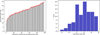 |
Fig. 11 100 realizations of spherical inclusions with random radii, at a fixed mass of 1 g (left: realizations ordered by dose rate, with 2-sigma error bars in red and right: histogram). |
5.4 Spherical inclusions with “cannonall” distribution
Different geometrical arrangements of dust in the cubic corner, created with the algorithm described in the Section 3.4, are simulated in order to model in a more realistic way the dust accumulated on the edges of the cube, like classical dust in a room. These geometrical arrangements of the dust also allow for a non-uniform packing fraction and variable average chord length distribution in the cube. Two of these geometric shapes are obtained by intersecting the cube either with an eighth of a sphere (sphere octant) or with three hyperbolic cylinders. All geometries are composed of 289 spheres of diameter 1 mm and ρ = 6.6 g/cm3, and have a total mass of 1 g. The equivalent dose rates (expressed in μSv/h) obtained are lower than those obtained with the classical RSA method of adding spherical inclusions (cf. Fig. 12).
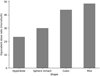 |
Fig. 12 Comparison between the dose rate obtained with different geometrical configurations, at constant mass of 1 g and density = 6.6 g/cm3. The detection point is at 15 cm from the centre of the original cubic corner. |
5.5 Dust aggregates simulation
Dust also accumulates in the form of aggregates. In the aggregate model, each aggregate is modelled by a dense assembly of twelve small spheres contained within a larger sphere. Several aggregates are randomly placed in a corner as described in Section 3.5. The density of each small sphere forming the aggregate is equal to the typical density of a MOX fuel ρMOX = 11.016 g/cm3.
In the homogenized spheres model, the radius of the large spheres in which the 12 small spheres are homogenized is the same as the radius of the large spheres containing the aggregates of 12 small spheres. The density of the homogeneous larger sphere is equal to the average density of the 12 spheres homogenized with the air contained in the sphere ρMOX × ξ12-packing spheres = 4.67 g/cm3. Simulations were performed with 1000 batches of 5000 particles to obtain a PRSD < 0.8%.
The equivalent dose rate obtained with this aggregate model is compared to that obtained with the model of small spheres homogenised in large spheres (cf. Fig. 13).
The equivalent dose rate obtained with the aggregate model with 12 small spheres is lower than that obtained with 12 homogenized spheres in a larger sphere. Indeed, instead of one large, less dense emitting sphere, the twelve smaller, denser emitting spheres increase the self-protection of the sources, and thus decrease the equivalent dose rate.
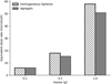 |
Fig. 13 Comparison between Gamma equivalent dose rate obtained with an inclusion of homogenized spheres and an inclusion of dense packing of 12 spheres inside a sphere of the same radius of the homogeneous one. |
6 Summary and conclusions
Tables 3 and 4 summarize the equivalent dose rate obtained with spherical inclusion dust grain models. In Table 3, the amount of dust is constant (1 g) and the radius of the spherical inclusion increases. In Table 4, the radius of inclusions is kept constant (0.05 cm) and the mass of dust, or the occupancy rate of the dust grains in a corner, increases.
The smaller the radius of the spheres modelling the dust grains, the more the equivalent dose rate increases and the closer the result is to the homogeneous model.
At constant radius, the lower the amount of dust, the further the model deviates from the homogeneous model.
In Table 5 are summarised the equivalent dose rate results obtained with the different stochastic dust models for a mass of 1 gram of dust deposited in a corner of the glove box.
Depending on the stochastic models used for the dust, the result differs more or less from the homogeneous model. The different strategies for explicit dust modelling give similar results, while they differ from the homogeneous model.
Homogeneous model can lead to grossly overestimate the dose on the hand of a glove box operator if dust has deposited in large aggregates in the corners of the box. Conversely, if a dose measurement in the glove box is used to deduce the amount a radioactive dust (as an inverse problem), the quantity of material can be greatly underestimated. For the specific application of radioprotection in a glove box that we considered in this paper, the two models with aggregates (cannonball and homogenized aggregates) are two extreme cases that bound the dose estimates: both of them should be simulated. The array of models presented in this paper gives tools to model different spatial configurations of dust grains and should be used accordingly.
Equivalent dose rate calculated for different values of the radius of the source spheres.
Equivalent dose rate calculated for different packing fractions.
Equivalent dose rate calculated with the different stochastic models.
Conflict of interests
The authors declare that they have no competing interests to report.
Funding
This research did not receive any specific external funding.
Data availability statement
Data associated with this article cannot be disclosed due to legal reason.
Author contribution statement
All authors have contributed to the general design of this work, to the computations and to the analyses. Alice Bonin and Coline Larmier have written the paper.
Acknowledgements
The authors thank the TRIPOLI-4® team and especially François-Xavier Hugot for his help in simulating the numerous sources with the transport code.
References
- C. Larmier, A. Zoia, F. Malvagi, E. Dumonteil, A. Mazzolo, Monte Carlo particle transport in random media: the effects of mixing statistics, J. Quant. Spectr. Radiat. Transfer 196, doi: 10.1016/j.jqsrt.2017.04.006 (2017) [Google Scholar]
- E. Brun, F. Damian, C.M. Diop, E. Dumonteil, F.X. Hugot, C. Jouanne, Y.K. Lee, F. Malvagi, A. Mazzolo, O. Petit, J.C. Trama, T. Visonneau, A. Zoia, Tripoli-4®, CEA, EDF and AREVA reference Monte Carlo code, Ann. Nucl. Energy 82, 151–160 (2015) [CrossRef] [Google Scholar]
- M.M.R. Williams, E. Larsen, Neutron transport in spatially random media: eigenvalue problems, Nucl. Sci. Eng. 139, Doi:10.13182/NSE01-A2222 (2001) [Google Scholar]
- F.B. Brown, W.R. Martin, Stochastic geometry capability in MCNP5 for the analysis of particle fuel, Ann. Nucl. Energy 31, 2039–2047 (2004) [CrossRef] [Google Scholar]
- V. Rintala, H. Suikkanen, J. Leppänen, R. Kyrki-Rajamäki, Modeling of realistic pebble bed reactor geometries using the Serpent Monte Carlo code, Ann. Nucl. Energy 77, 223–230 (2015) [CrossRef] [Google Scholar]
- M.M.R. Williams, Some aspects of neutron transport in spatially random media, Nucl. Sci. Eng. 136, 34–58 (2000) [CrossRef] [Google Scholar]
- C. Larmier, E. Dumonteil, F. Malvagi, A. Mazzolo, A. Zoia, Finite-size effects and percolation properties of Poisson geometries, Phys. Rev. Energy 94, 012130 (2016) [Google Scholar]
- C. Larmier, A. Zoia, F. Malvagi, E. Dumonteil, A. Mazzolo, Neutron multiplication in random media: reactivity and kinetics parameters, Ann. Nucl. Energy 111, 391–406 (2018) [CrossRef] [Google Scholar]
- A. Marinosci, C. Larmier, A. Zoia, Neutron transport in anisotropic random media, Ann. Nucl. Energy 118, 406–413 (2018) [CrossRef] [Google Scholar]
- P. Boulard, C. Larmier, J.C. Jaboulay, A. Zoia, J.M. Martinez, Neutron multiplication in fuel-water random media, in ICNC 2019-11th International conference on Nuclear Criticality Safety, September 15-20, Paris, France (2019) [Google Scholar]
- G.C. Pomraning, Linear kinetic theory and particle transport in stochastic mixtures (World Scientific Publishing, NJ, USA, 1991) [Google Scholar]
- C. Larmier, Stochastic Particle Transport in Disordered Media: beyond the Boltzmann Equation, PhD Thesis, Paris-Saclay University 9–18, 25–27 (2018) [Google Scholar]
- D.C. Irving, The adjoint Boltzmann equation and its simulation by Monte Carlo, Nucl. Eng. Des. 15, 273 (1971) [CrossRef] [Google Scholar]
- D. Haas, A. Vandergheynst, J. Van Vliet, R. Lorenzelli, J.L. Nigon, Mixed-oxide fuel fabrication technology and experience at the Belgonucléaire and FCCa plants and further developments for the Melox plant, Nucl. Technol. 106, 77–81 (1994) [Google Scholar]
- J.L. Nigon, G. Le Bastard, Fabrication des combustibles au plutonium, Techniques de l'Ingénieur, traité Génie Nucléaire, Réf. BN3630 V1 (2002) [Google Scholar]
- M.D. Dorrian, M.R. Bailey, Particle size distribution of radioactive aerosols measured in workplaces, Radiat. Protect. Dosim. 60, 119–133 (1995) [CrossRef] [Google Scholar]
- E. Ansoborlo, Particle size distributions of uranium aerosols measured in the French nuclear fuel cycle, Radioprotection 32, 319–330 (1997) [CrossRef] [EDP Sciences] [Google Scholar]
- K. Vishwa Prasad, A.Y. Balbudhe, G.K. Srivastava, R.M. Tripathi, V.D. Puranik, Aerosol size distribution in a uranium processing and fuel fabrication facility, Radiat. Protect. Dosim. 140, 357–361 (2010) [CrossRef] [Google Scholar]
- E. Ansoborlo, V. Chazel, M.H. Hengé-Napoli, P. Pihet, A. Rannou, M.R. Bailey, N. Stradling, Determination of the physical and chemical properties, biokinetics, and dose coefficients of uranium compounds handled during nuclear fuel fabrication in France, Health Phys. 82, Number 3 (2002) [Google Scholar]
- P. Fritsch, K. Guillet, Granulometry of aerosols containing transuranium elements in the workplace: an estimate using autoradiographic analysis, Ann. Occup. Hyg. 46, 292–295 (2002) [Google Scholar]
- P. Massiot, B. Leprince, C. Lizon, L. Le Foll, I. L'Huillier, G. Rataeu, P. Fritsch, Physico-chemical characterisation of inhalable MOX particles according to the industrial process, Radiat. Protect. Dosim. 79, 43–47 (1998) [CrossRef] [Google Scholar]
- T. Kravchik, S. Oved, O. Paztal-Levy, O. Pelled, R. Gonen, U. German, A. Tshuva, Determination of the solubility and size distribution of radioactive aerosols in the uranium processing plant at NRCN, Radiat. Protect. Dosim. 131, 418–424 (2008) [CrossRef] [Google Scholar]
- E. Hansson, H.B.L. Pettersson, C. Fortin, M. Eriksson, Uranium aerosols at a nuclear fuel fabrication plant: Characterization using scanning electron microscopy and energy dispersive X-ray spectroscopy, Spectrochim. Acta B 131, 130–137 (2017) [CrossRef] [Google Scholar]
- G. Sengler, EPR core design, Nucl. Eng. Des. 187, 79–119 (1999) [CrossRef] [Google Scholar]
- A. Tsilanizara, C.M. Diop, B. Nimal, M. Detoc, L. Lunéville, M. Chiron, T.D. Huynh, I. Brésard, M. Eid, J.C. Klein, DARWIN: an evolution code system for a large range of applications, J. Nucl. Sci. Technol. 37, 845–849 (2000) [CrossRef] [Google Scholar]
- A. Koning, R. Forrest, M. Kellet, R. Mills, The JEFF-3.1 Nuclear Data Library, JEFF Report 21 − OECD (2006) [Google Scholar]
- R. Kinsey, ENDF-102, Data Formats and Procedures for the Evaluated Nuclear Data File, ENDF, BNL-50496 2nd Edition, Brookhaven National Laboratory (October 1979), revised by B. Magurno (November 1983) [Google Scholar]
- International Commission on Radiological Protection, 2007. The 2007 Recommendations of the International Commission on Radiological Protection. ICRP Publication 103. Ann. ICRP Vol. 37 (2–4) (Elsevier) (2007) [Google Scholar]
- ICRU, International Commission on Radiation Units and Measurements, Quantities and Unit in Radiation Protection Dosimetry. ICRU Report 51 (ICRU, 7910 Woodmont Avenue, Suite 800, Bethesda, MD, 1993) [Google Scholar]
- S. Torquato, Random heterogeneous materials: microstructure and macroscopic properties (Springer-Verlag, New York, USA, 2013) [Google Scholar]
- B. Widom, Random sequential addition of hard spheres to a volume, J. Chem. Phys. 44, 3888 (1966) [CrossRef] [Google Scholar]
- H. Pfoertner, Densest packing of spheres in a sphere (2013). Available at www.randomwalk.de/sphere/insphr/spheresinsphr.html. Accessed October 6, 2020 [Google Scholar]
- T. Gensane, Dense packings of equal spheres in a larger sphere, Les Cahiers du LMPA J. Liouville 188, June 2003 [Google Scholar]
- P.S. Brantley, J.N. Martos, Impact of spherical inclusion mean chord length and radius distribution on three-dimensional binary stochastic medium particle transport, in Proceedings of M&C 2011, Rio de Janeiro, Brazil (2011) [Google Scholar]
- A. Mazzolo, B. Roesslinger, Monte-Carlo simulation of the chord length distribution function across convex bodies, non-convex bodies and random media, Monte Carlo Meth. Appl. 10, 443–454 (2004) [CrossRef] [Google Scholar]
Cite this article as: Alice Bonin, Matteo Zammataro, Coline Larmier, Modelling of radioactive dust for dose calculations with stochastic geometries, EPJ Nuclear Sci. Technol. 8, 6 (2022)
All Tables
RSA spherical inclusion method, equivalent dose rate (EDR) calculated for different values of the radius of the source spheres.
Equivalent dose rate calculated for different values of the radius of the source spheres.
All Figures
|
Fig. 1 Visualisation of sections of the glove box model obtained with TRIPOLI-4® viewer: (y,z) plane on the left, and (x,z) plane on the right. The red cone represents the mixed oxide in the jar, the red rectangle in the centre the pressing table and the cross at the bottom right the corner full of dust, just behind the Kyowa Glass (in green in the figure). |
| In the text | |
|
Fig. 2 Simulation of the corner of the glove box with spherical inclusions. |
| In the text | |
|
Fig. 3 Representation of the geometry obtained from the intersection of the original cube with 3 hyberbolic cylinders for 5 g of spherical inclusions with a radius of 0.025 cm. |
| In the text | |
|
Fig. 4 Drawing of the dense 12 spheres hexagonal close packing inside a bigger sphere (source: https://en.wikipedia.org/wiki/Sphere_packing_in_a_sphere). |
| In the text | |
|
Fig. 5 Homogeneous model, Corner source with parametrical variation of the density, results at 15 cm from the source. |
| In the text | |
|
Fig. 6 Homogeneous model, Corner source with parametrical variation of the density, results right over the press. |
| In the text | |
|
Fig. 7 RSA spherical inclusion method, Gamma simulations with different values of the sphere radii with a constant mass of 1g for each corner and constant density of 6.6 g/cm3 (relative standard deviation inferior to 1%, given in Tab. 2, are not presented on the figure). |
| In the text | |
|
Fig. 8 Spherical inclusion model, Gamma simulation with spheres of constant radius of 0.05 cm, constant density of 6.6 g/cm3 and variable packing fraction (PRSD are inferior to 1%). |
| In the text | |
|
Fig. 9 Spherical inclusion model, neutron simulation with spheres with a fixed constant radius of 0.05 cm and a constant density of 6.6 g/cm3 with variable packing fraction (PRSD are inferior to 1%). |
| In the text | |
|
Fig. 10 100 realizations of spherical inclusions with R = 0.05 cm, ξ = 0.00121 and ρMOX = 6.6 g/cm3 (left: realizations ordered by dose rate, with 2-sigma error bars in red and right: histogram). |
| In the text | |
|
Fig. 11 100 realizations of spherical inclusions with random radii, at a fixed mass of 1 g (left: realizations ordered by dose rate, with 2-sigma error bars in red and right: histogram). |
| In the text | |
|
Fig. 12 Comparison between the dose rate obtained with different geometrical configurations, at constant mass of 1 g and density = 6.6 g/cm3. The detection point is at 15 cm from the centre of the original cubic corner. |
| In the text | |
|
Fig. 13 Comparison between Gamma equivalent dose rate obtained with an inclusion of homogenized spheres and an inclusion of dense packing of 12 spheres inside a sphere of the same radius of the homogeneous one. |
| In the text | |
Current usage metrics show cumulative count of Article Views (full-text article views including HTML views, PDF and ePub downloads, according to the available data) and Abstracts Views on Vision4Press platform.
Data correspond to usage on the plateform after 2015. The current usage metrics is available 48-96 hours after online publication and is updated daily on week days.
Initial download of the metrics may take a while.