| Issue |
EPJ Nuclear Sci. Technol.
Volume 7, 2021
|
|
|---|---|---|
| Article Number | 8 | |
| Number of page(s) | 13 | |
| DOI | https://doi.org/10.1051/epjn/2021006 | |
| Published online | 07 April 2021 | |
https://doi.org/10.1051/epjn/2021006
Regular Article
A multivariate representation of compressed pin-by-pin cross sections
Université Paris-Saclay, CEA, Service d’Études des Réacteurs et de Mathématiques Appliquées,
91191
Gif-sur-Yvette, France
* e-mail: This email address is being protected from spambots. You need JavaScript enabled to view it.
Received:
3
September
2020
Received in final form:
12
February
2021
Accepted:
3
March
2021
Published online: 7 April 2021
Abstract
Since the 80’s, industrial core calculations employ the two-step scheme based on prior cross sections preparation with few energy groups and in homogenized reference geometries. Spatial homogenization in the fuel assembly quarters is the most frequent calculation option nowadays, relying on efficient nodal solvers using a coarse mesh. Pin-wise reaction rates are then reconstructed by dehomogenization techniques. The future trend of core calculations is moving however toward pin-by-pin explicit representations, where few-group cross sections are homogenized in the single pins at many physical conditions and many nuclides are selected for the simplified depletion chains. The resulting data model requires a considerable memory occupation on disk-files and the time needed to evaluate all data exceeds the limits for practical feasibility of multi-physics reactor calculations. In this work, we study the compression of pin-by-pin homogenized cross sections by the Hotelling transform in typical PWR fuel assemblies. The reconstruction of these quantities at different physical states of the assembly is then addressed by interpolation of only a few compressed coefficients, instead of interpolating separately each homogenized cross section. Savings in memory higher than 90% are observed, which result in important gains in runtime when interpolating the few-group data.
© D. Tomatis, published by EDP Sciences, 2021
 This is an Open Access article distributed under the terms of the Creative Commons Attribution License (https://creativecommons.org/licenses/by/4.0), which permits unrestricted use, distribution, and reproduction in any medium, provided the original work is properly cited.
1 Introduction
The preparation of homogenized cross sections in a few energy groups is a very practical and effective approach, extensively used nowadays for core calculations. The basic geometry in which the cross sections are homogenized is the fuel element. Quarters of fuel assemblies are generally used in LWR as cells for a coarse mesh, whereas VVER and fast reactors choose hexagonal sectors. The choice is driven by the kind of reference frame depicted by the lattice of the fuel rods.
Regarding core calculations, the neutron population is described by a low-order transport approximation, like diffusion [1], where the input data are the homogenized cross sections. Concisely, homogenization consists of the particular integration of the reaction rates in energy, angle and space with a reference flux solution from transport. Homogenized cross sections follow then by dividing the reaction rates by the flux integrated over the same portion of the phase space. This reference flux is calculated in idealized conditions, and assumed valid for more general configurations such as those occurring during reactor operation. However, the real conditions of operation of the fuel element once loaded into the core remain totally unknown. The same procedure generating these data is then applied to all types of fuel elements considered for the core plan. This approach is at the base of a homogenization paradigm [2].
Of course, the physics of diffusion and the physics of transport, which is the true one governing the real behavior of neutrons in the lattice, are different. They do not reproduce in general the same leakage rates, even when the reaction rates are preserved. Therefore a calibration of the process of data generation is necessary by recurring to Equivalence theory, which enforces the equivalence between transport and diffusion on reference leakage and reaction rates after homogenization. In particular, Equivalence theory can request the use of additional coefficients to store as in the case of the assembly discontinuity factors [3]. This supplementary storage need can be avoided if the super-homogenization (SPH) factors are used, but at the cost of a longer data preparation and with fewer degrees of freedom to adjust the solution [1]. In fact, discontinuity factors are defined on cell surfaces with one value per face, while a single SPH coefficient per cell is sufficient. The calculation of the SPH factors is iterative by definition, being the reason for the longer overall preparation.
The trend of designing more heterogeneous reactors and the continuous goal to achieve higher physical accuracy for the distribution of the reaction rates is progressively orienting the development of neutronics computer codes towards pin-by-pin capabilities. Although the progress in parallel computers allows faster calculations, the data model instructing the multi-physics coupling with thermal-hydraulic codes still needs a considerable amount of storage on disk-files. At the same time, this means also a significant overhead in the computation of the few-group cross sections by interpolation when taking into account the new updated thermal variables. Specifications of a typical pin-by-pin cross section model follow in Section 2.
In this work we apply the Hotelling transform (HT) to reduce the potential redundancy in the cross section data, see Section 3, and we propose to interpolate only a few compressed coefficients for reconstructing the full set of pin-wise homogenized cross sections. The accuracy of the new compressed data set after truncated compression is discussed in Section 4. The HT allowed savings up to 90% in a previous work about power form factors [4], which originally suggested in the conclusion the idea of interpolating the compressed coefficients of homogenized cross sections. No mathematical argument was provided though to demonstrate the feasibility of this idea. The HT was also applied successfully with pin-by-pin 3D burnup data by testing different types of matricization on the initial multidimensional data set [5]. However, these works focused only on the compression of different data sets without introducing function approximation to reconstruct information from the reduced model. The application of a linear interpolation problem yet in the transformed space is explained in Section 5, demonstrating mathematically the interest in this approach. A limited number of compressed coefficients can then be interpolated on the stateparameters to yield the updated cross sections for the thermal reactivity feedback by the inverse transform. Of course, this aims achieving a reduction in the global runtime with respect to interpolating each cross section separately. The methodology is applied in Section 6 with pin data prepared on two PWR fuel assemblies from a known benchmark problem [6]. Finally, conclusion follows in Section 7.
2 Specifications of the pin-by-pin data model
The nuclear cross sections are homogenized in each pin cells of the fuel assembly and condensed to the few-group energy formalism selected for the core flux solver. This procedure is executed at many different physical conditions in order to describe the neutronics response of the fuel assembly. Each physical condition is identified by a list of state parameters, which are the most important quantities affecting the neutron reactivity of the system. Among these variables, there is for instance the temperature in the fuel, reproducing the well-known Doppler effect of resonance broadening. The thermo-dynamic state of the coolant is also represented in thermal reactors with neutron moderation by water. Two variables are needed in case of sub-cooled convection, and void is introduced with di-phasic flow regimes. The concentrations of the main neutron absorbers, like diluted boron in water in PWR or xenon produced in the fuel pellets, can also be used as state parameters. Basically, the choice of the state parameters is reactor-dependent, characterizing the reactor itself, and determined by the types of reactivity feedback reproducing its physical behavior.
Each assembly is calculated in presumed conditions of operation, since the actual operating conditions cannot be known in advance. It is then considered as surrounded by other assemblies, which are usually of the same type so that reflection applies at the boundary. These calculations are performed by exposing the fuel element up to a target burnup and at a constant power level. Only the microscopic cross sections of a few nuclides are prepared because burnup calculations operated at the core level use simplified decay chains to achieve global runtime optimization. The preparation of separate data per nuclide allows to consider different spectral conditions for fuel depletion when the element is placed into the core. The concentrations of these special nuclides along the core cycle are computed by using reaction rates determined by the core solver. These rates are actually computed with homogenized microscopic cross sections interpolated on lookup tables at the local values of the state parameters. The spatial description in the core of these nuclides affects sharply the storage need. This motivates the simplifications in the depletion chain and the practical usage of lumped nuclides, which are fictitious materials whose compounds’ concentrations are bound by constant ratios. They are used for groups of fission products and burnable poisons. Instead, the main actinides must always be treated separately for applications with long cycle exposure and high flux irradiation. 135Xe and 135I are needed for instance to study the power fluctuations due to short-term control. About PWR, 10B is included because it is responsible for long-term control. A residual material lumps all other nuclides which are not considered by the depletion solver of the core code. Dedicated algorithms produce the simplified decay chains after selection of the number of nuclides to track in the core calculation.
Cross sections are homogenized over the Cartesian grid defined by the physical cells of the lattice, yielding the final pin-by-pin representation with a homogeneous mixture per cell. It must be noted again that the postulated physical conditions for lattice calculations are quite approximate, with reflection at the boundary as main strong assumption. Moreover, the temperature in the fuel is distributed uniformly as a simplification to avoid expensive iterations between the lattice computer code and a thermo-mechanical code.
3 Compression by redundancy reduction
The main goal of data compression is the reduction in the storage need [7]. Different representations of the actual data are sought with compression algorithms by removing hidden redundancy and by extracting the only relevant components. Compression can occur with minimal or controlled loss of information, or it can keep the full original content. We talk of lossy compression in the first case, lossless in the second one. A compression algorithm includes several steps, with a numerical transform as key element. Quantization and further encoding may follow with specific features that depend on the particular use, like with the online processing of videos and images. Here, we focus our attention on the Hotelling transform, which showed the best compression performances in previous works [4, 5].
The different assembly states are calculated by several lattice transport calculations. Each calculation corresponds to a given combinationof P parameters, which are considered as linearly independent in a multi-dimensional space  built by the Cartesian composition of the sets ofreal points
  , so that
  with
with  , ∀i. The few-group partial cross sections are then considered as functions of the state parameters, i.e.
  . They are known only at the points of the hyper-rectangular grid composed by
 ![Mathematical equation: $[p_{1,\pi_1}, \pi_1 = 1, \ldots, \Pi_1] \times \ldots \times [p_{P,\pi_P}, \pi_P = 1, \ldots, \Pi_P]$](/articles/epjn/full_html/2021/01/epjn200019/epjn200019-eq6.png) , for a total of
, for a total of  state points.Besides, they are strictly positive real-valued functions.
Regardless of the microscopic or macroscopic attribute, that is in practice linking the intended cross section to a non-unitary nuclide concentration, pin-wise cross sections can be represented by multi-dimensional arrays with elements like σ(k, π1, …, πP). The new index k refers to thepin position in the assembly, after unfolding all pins by the lexicographical order for instance. When appropriate, the array can be extended with more dimensions to account also for the type of nuclide or for the typeof partial reaction in order to represent more microscopic cross sections under the same entity in memory. In this case, the dependencies other than the state parameters can still be arranged along the k-th axis.
We now reshape the previous array in order to get the real-valued matrix ![Mathematical equation: $\mathbf{M} = [m_{k,q} = \sigma(k,q), k=1, \ldots, K, q=1, \ldots, \cal{P}]$](/articles/epjn/full_html/2021/01/epjn200019/epjn200019-eq8.png) , where the original array has been flattened on the p’s axes using the column-major order for the second dimension, such that q = π1 + Π1(π2 + Π2(…(πP−1 + ΠP−1πP)…)). A similar result can be obtained by flattening with the row-major order. The shape of M becomes
, where the original array has been flattened on the p’s axes using the column-major order for the second dimension, such that q = π1 + Π1(π2 + Π2(…(πP−1 + ΠP−1πP)…)). A similar result can be obtained by flattening with the row-major order. The shape of M becomes  , being K the number of pin cells in the assembly for instance. The size of M
  is expected to be very large.
After centering the matrix around the mean by columns m⃗, that is by the operation  , we can obtain the covariance matrix by the scalar product with its transpose, i.e. C = Z ⋅ZT∕K.
  is a vector of all ones and length
  . The above column-wise mean stands for the expected value of each cross section over the state parameter space
  , provided unitary distributions, i.e.
  . The expansion of the covariance matrix in terms of the components of Z yields simply
  .
.
In order to apply the HT we must resolve the following eigenvalue problem:
 (1)
(1)
with the eigen-vectors arranged by column in E and the eigenvalues λ along the diagonal matrix Λ. The matrix E is unitary after proper normalization, i.e. E T = E−1. Since the covariance matrix is real and symmetric by definition (CT = C), thus Hermitian positive semi-definite, the eigenvalues are all real. They can be computed for instance by a fast divide-and-conquer algorithm [8], like by the LAPACK routine syev [9]. These eigenvalues represent the variances in the transformed space where the new coordinates are de facto completely decorrelated. So the HT consists in determining the new coordinates:
 (2)
(2)
whose covariance matrix is again Λ. The inverse transform follows simply by multiplying equation (2) with E from the left and by summing the mean values:
 (3)
(3)
The HT of the matrix M requires the solution of an eigenvalue problem for the square covariance matrix, whose size is K2, and the computational effort is small for  . Otherwise, recurring to the singular value decomposition (SVD) of Z can be a better choice [8]. In fact, by Z = USV, with the left singular vectors in U, the right singular vectors in V and the singular values along the main diagonal of S, it follows that KC = Z ⋅ZT = US2UT. The squared singular values yield then the sought variances, and the singular vectors the matrix E. SVD can also be computed fast by the divide-and-conquer algorithm, like by the LAPACK routine gesdd.
After sorting the eigen-pairs by decreasing order of the corresponding eigenvalues (or singular values), it is possible to truncate the decomposition by neglecting the terms associated to the lowest variances. The truncation yields of course an approximation of the original matrix M, say M′, leading to acontrolled lossy compression. The new quantities to store are the transformed coefficients in Y, the transformed directions in E and the mean values in m⃗. Sometimes, it can be numerically beneficial to divide the samples by the standard deviation (Std), still computed by columns. In this case the same equations introduced so far apply after the redefinition M ←S−1M, with  and
and ![Mathematical equation: $^{\rightarrow}{\cal{s}} = \operatorname{Std}([\sigma(k,{\bullet}), k=1, \ldots, K]) = (\mathbf{M}^{\{2\}} \cdot ^{\rightarrow}{1}_{\cal{P}} / \cal{P} - ^{\rightarrow}{m}^{\{2\}})^{\{\,^{1}\!/_{2}\}}$](/articles/epjn/full_html/2021/01/epjn200019/epjn200019-eq22.png) , where
, where  stands for the element-wise exponentiation to the power N. An additional matrix multiplication is also needed after the inverse transformation, and the storage cost increases of one more array of size K. It must be noted that the matricesY and E become rectangular after truncation. Many eigenvalues can be neglected in general thanks to the high decorrelation capability of the HT, thus achieving high compression. Actually, neighboring samples can be highly correlated in the original data representation, meaning hidden redundancy that compression seeks to reduce.
The compression performances are given by the compression ratio CR, determined by the initial number of values to store over the final number of compressed coefficients retained. The CR is related to the memory savings μ = 1 − 1∕CR, assuming the same floating point representation in memory for the data. After keeping κ variances at truncation (out of the available K), the CR is determined as:
![Mathematical equation: \begin{equation*} \textrm{CR} = \frac{K \cal{P}}{K \kappa + \kappa \cal{P} + 2K} = \left[ \frac{\kappa + 2}{\cal{P}} + \rho \right]^{-1}\end{equation*}](/articles/epjn/full_html/2021/01/epjn200019/epjn200019-eq24.png) (4)
(4)
with ρ = κ∕K < 1. Equation (4) considers two matrices and two arrays to store because of the transform, that is using also the normalization of the original data by the standard deviation. It is possible to notice that CR ≈ 1∕ρ for  , which is the case of a dense sampling in
  , or when the system is characterized by several types of reactivity feedback, implying many independent state parameters. Moreover, savings in storage occur only for
 (5)
(5)
We can recognize the fraction  as the minimal fraction of rows to remove over the original K rows to have a positive storage gain.
The mean squared error between the original data and the approximated data can be determined by the Frobenius norm, becoming equal to the sum of the discarded variances by virtue of the properties of unitary matrices, see [4] for a short demonstration. For completeness, the Frobenius norm of a matrix is defined as the squared root of the sum of all its squared elements in absolute value. This norm bounds the maximum element-wise norm [8]:
 (6)
(6)
with the error matrix R = M −M′ and after retaining the first κ variances and modes (out of the available K). Obviously, zero error corresponds to compression without truncation, and vice versa. If all K terms are truncated, ∥R∥F matches ∥M∥F given by thesum of all variances, or by the sum of its squared singular values, with 100% error. We estimate the relative error by ∥R ∥F∕∥M∥F and we say that M′ approximates M to d decimal digits if the relative error is O(10−d).
4 Remarks about accuracy of compressed cross sections
The process of cross section preparation involves many approximations and assumptions, yet regardless of the possible simplifications in the calculation schemes introduced to have shorter runtime at execution. The first and foremost approximation concerns reflection at the boundary of the modelled assembly, which applies all along the burnup calculation. This condition is accepted despite it is certainly not met at real operation. Hence, the homogenized cross sections must always be considered as approximated quantities in the context of core calculations, even when the reaction rates are preserved in the modelled fuel assembly by lattice calculations.
The application of a numerical transform like HT on a set of cross sections yields an equivalent representation, since the only loss in accuracy may come from the numerical precision of the machine, which is generally not a severe issue with modern computers and floating point arithmetic. Loss in accuracy does come afterwards when truncating the sum of the eigen-decomposition. Although experience shows that many terms can usually be removed with limited loss of initial information, it is necessary to provide recommendations for acceptable tolerances on the quantities of interest, being still the reaction rates.
When considering the reaction rates calculated by the lattice transport calculation, the accuracy of the reconstructed rates is determined by the only reconstructed cross sections, since the condensation flux is known and it can be considered as a reference. Instead, when considering the reaction rates calculated later in a core calculation, the mutual relation between the cross sections and the flux must be taken into account. The derivatives of the reaction rates, or say their incremental variations, on the homogenized cross sections should be measurable to fix precise thresholds at truncation. First-order Perturbation Theory can avoid the calculation of new flux distributions with the modified cross sections, but a transport operator is needed. It seems natural to adopt the low-order operator selected for Equivalence Theory, which is required anyway in both pin-by-pin or assembly-quarter representations. But in case equivalence is applied, it could even correct the error in the truncated cross sections. For instance, SPH equivalence corrects the local cross sections to match the reference reaction rates. Equivalence is usually included in the initial preparation process, but it can also be called at a second stage, that is on demand right before setting up a core calculation, like when rehomogenization techniques are used for the cross sections. This would require the additional storage of a few macroscopic reference reaction rates per assembly, which is however much smaller than the whole microscopic dataset. We set apart these considerations hereafter in favor of a simpler argument, based on the neutron reactivity.
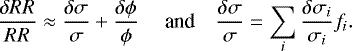
The infinite multiplication factor of the fuel assembly is calculated as k∞ = PR∕AR, with the total neutron production and absorption macroscopic reaction rates, PR and AR, respectively, of the kind σϕ. The neutron fluxϕ is volume-integrated. This notation implies the sum of the rates in all pin cells, which are still computed in the assembly with reflection at the boundary. These are integral rates in energy and space. As well, the absorption cross section is used for AR, while PR uses the fission cross section times the neutron multiplicity. If we indicate a variation of a reaction rate RR as δRR = RR′− RR, with the prime to indicate the modified state, we can express the change in reactivity at first-order as:
 (7)
(7)
with both relative differences given in the form:
 (8)
(8)
The cross section change is further decomposed in the sum of its microscopic components over the available nuclides with the fractions fi = Niσi∕σ, being Ni the nuclide density. The flux change is expected in opposite sign for a change in absorption and production for physical reasons, but exact compensation of their effects is rare or plainly unrealistic. As an example, this simple derivation shows that 1% change in the production rate can cause a deviation of 1000 pcm in reactivity. The uncertainty on reactivity computed by lattice calculations is typically around ±50 pcm, which means 0.05% tolerable differences on rates. The microscopic cross sections can however be treated differently according to the fraction fi, that relaxes this strict requirement. In other words, higher truncation error can be accepted on the cross sections of a nuclide that is contributing less to the corresponding macroscopic cross section. The separate treatment of the nuclides for a lossy compression affects the definition of the matrix M with proper grouping of the indices other than p⃗ under the index k.
Another solution to assess sensitivity of reaction rates on cross sections would be to perform assembly calculations with different nuclear data libraries. This option is dropped out in this work because it would demand too many expensive and long calculations.
5 Multivariate polynomial interpolation
The reconstruction of the few-group cross section data as continuous functions over  is usually performed by a linear interpolation scheme [10–12]. Here, cross sections are always considered as homogeneous data in each cell of the spatial mesh used for the calculation.
Specifically, this means constructing an approximation s to a given cross section σ in the form 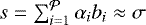 , with the real coefficients αi and known functions bi defined on the same domain
  of σ [13]. The particular approximation by interpolation is achieved by the linear functionals
  , describing different interpolation conditions:
 (9)
(9)
Hence, the approximation problem depends only on the linear span of the expansion functions and on the linear span of the interpolation conditions, i.e. {∑iαibi} and {∑iαiγi}, respectively, with  for both sets. Although ordinary interpolation is used in the following, being
  , the same conclusion holds with many other schemes, like osculatory interpolation or least-squares approximations for instance. We select a polynomial base in this work for the expansion functions, using tensor products of linear spaces of univariate functions.
The linear interpolation problem derived from the system equations in (9) has a unique solution if and only if the Gramian matrix ![Mathematical equation: $\mathbf{G} = [\gamma_i b_j, \; i,j=1, \ldots \cal{P}]$](/articles/epjn/full_html/2021/01/epjn200019/epjn200019-eq39.png) is invertible, in order to obtain the fitting coefficients by
is invertible, in order to obtain the fitting coefficients by
 (10)
(10)
with ![Mathematical equation: $^{\rightarrow}{\gamma} = [\gamma_i, \; i=1, \ldots, \cal{P}]$](/articles/epjn/full_html/2021/01/epjn200019/epjn200019-eq41.png) and α⃗ containing all αi.
and α⃗ containing all αi.
The dependence of the cross sections on the state parameters reproduces the reactivity feedback in the neutron multiplying system. This is a fundamental point for multi-physics calculations employing the two-level scheme based on Homogenization and Equivalence theory [1]. The computational cost associated to the function evaluation of all cross section approximations becomes rapidly excessive as soon as the calculation model is enhanced with more nuclides and further refinement is operated on the initial coarser mesh in space. For example, the pin-by-pin partition of the assembly lattice implies tracking the same isotope in every pin during the burnup calculation, instead of using a single quantity averaged in its volume, that is with only one cell per assembly. This often forces the use of constant values for the state parameters on multiple cells in order to reduce the total number of function evaluations, thus accepting simplified and surrogated physical models in the coupled problem, or a loss of information obtained by computationally expensive solvers. In the former case, the computer codes which require more computational resources could be penalized by poor physical information coming from the other codes, without significant gain in the global accuracy. In the latter case, the thorough and costly efforts spent could be cancelled by subsequent averaging. Eventually, the introduced simplifications may not be worth the total computational cost.
It is then necessary to find a solution allowing to keep the ensued degree of physical description and accuracy in the coupled problem. Byvirtue of linearity indeed, the interpolation scheme can be applied directly onto the compressed coefficients, after applying the HT on the output space created by a collection of cross sections, as shown in Section 3:
 (11)
(11)
It is assumed implicitly in equation (11) that linear interpolation does not alter constant values. The modes (singular vectors) in the matrix E are not subject to interpolation because E commutes with the application of the linear functionals vector.
The size of the matrix Y with the transformed coefficients is  , where κ < K is the number of the only variances retained by truncation. Its elements laying on the second dimension retain the dependencies on the state parameters at the coordinates πi, i = 1, …, P. The reverse reshaping of each row of Y to recover separate indices per axis
  yields the new multi-dimensional arrays for extending σ continuously on
  by multivariate interpolation. The total computational cost for interpolation is thus reduced theoretically by the ratio ρ used for equation (4), since the matrix multiplication by the (only) rectangular portion of E, the sum with the mean values and the multiplication by the standard deviations take negligible time. Hence the higher the efficiency at compression, the faster the whole evaluation of the data set by interpolation.
6 Results
This section presents the results of the compression algorithm applied on two different multi-parameter datasets. The datasets contain two-group pin-by-pin homogenized cross sections prepared by lattice transport calculations performed with the code APOLLO3® v.2.0.2 [14]. Two PWR configurations are considered, coming from the benchmark problem proposed by Yamamoto [6]. The first configuration (UGd) is about a UO2 fuel assembly with some fuel pins poisoned by gadolinium, while the second one (MOX) uses mixed oxide fuel types. Both configurations show a heterogeneous lattice design. Cross sections of heavy nuclides are self-shielded by the fine structure method, also known as Livolant-Jeanpierre method, while the flux calculations are performed by the method of characteristics. The full problem specifications and calculation options are the same as in [4], hence we refer to the cited reference without repeating here all the details. A discussion about the application of the linear interpolation problem onto the compressed coefficients completes the section.
6.1 Dataset characterization
The two assemblies are calculated up to the average burnup of 70 GWd/t at constant thermal power, and the nuclide inventory determined at different times along the exposure is used to setup new calculations by varying the other state parameters. Table 1 shows the lists of values used for the different parameters. The list of burnup values is specified according to the input practice of APOLLO3® which needs a sequence of couples where the first key is the number of equally spaced points between the succeeding burnup values in the second keys. The burnup value list always starts from zero. The calculations at perturbed conditions are performed when the average burnup of the fuel assembly matches one of the values in this list. The finer burnup mesh in the last row of the table is used by the predictor-corrector scheme of the depletion solver. Temperature is set uniformly in the fuel and moderator regions. Natural abundances are used for 10 B and 11 B present in boric acid H3 BO3, which is diluted in the neutron moderating water. The values in bold are used to set the conditions of depletion at nominal operation along fuel exposure. The state parameter space spanned by these value lists is assumed covering operational conditions and reactivity-initiated accidents, with a total of 2850 calculation points.
Cross sections are condensed in two energy groups, whose bounds are in decreasing order: 19.64, 6.25E−07, and 1.10E−10 MeV; according to common usage, the first group is for fast neutrons while thermal neutrons are represented by the second one. Here we only consider two-group data sets to comply with standard core calculations using neutron diffusion theory that are performed in industry for reactor design and safety. Therefore, we consider only the reactions absorption, production (nu-fission) and scattering in the following, since the fission emission spectrum is fixed with non-zero (and unitary) neutron emission only in the fast group, and the other ones do not enter the neutron balance equation to solve. Cross sections are homogenized in each pin cell, producing microscopic cross sections for the following list of nuclides: 234−238U, 237,239Np, 238−242Pu, 241,242M,243Am, 242−245Cm, 135 I, 135 Xe, 149 Pm, and 149 Sm. Only one lumped residual is considered, even in the case of the gadolinium-poisoned assembly. Although this nuclide list is rather short, it can offer an idea of general use in reactor analysis and it serves the purpose of this work. The memory savings sought by the compression technique are expected to be proportional to the number of nuclides used.
The pin-wise distributions of homogenized cross sections are quite regular with higher variations around the spatial average at the beginning of the irradiation period due to the heterogeneity features of the assembly design. In the UGd fuel assembly for instance, the pin-wise distribution of thermal nu-fission cross section of 235 U shows a larger standard deviation with fresh fuel, see Figure 1, and consequent decrease of its average value for the presence of highly poisoned fuel pins, which have also a lower enrichment (4% instead of 6.5% in weight). Each point in the figure corresponds to a pin-wise distribution at a given physical state of the assembly. The values are plotted with dots changing color from black to red as far as the assembly is depleted (white standing in the medium range of exposure). The pin-wise distribution narrows with increasing averages after consumption of the poison and redistribution of the power through the pins of different fissile credits. Instead, the cross section of 235U for fast neutronproduction varies little in this assembly, with moderate increase of the average value at high burnup for plutonium build-up and spectrum hardening.
Thermal absorption of 238U in Figure 2 shows the same trend of thermal production of 235 U, contrary to its fast absorption that changes much less, but still with increasing mean when the spectrum hardens. The similar trends noticed with thermal cross sections in Figures 1 and 2 can be explained by the fact that both cross sections show the characteristic behavior of inverse proportionality to the neutron velocity (v) in the thermal range, being then averaged with a Maxwellian-like neutron spectrum at the same temperature.
We plot the absorption cross section of 239Pu from the MOX fuel assembly in Figure 3 as last example. Although three types of fuel pins with different plutonium content are used, the MOX fuel assembly shows less variability in space for the pin-wise distributions of the cross sections, and this holds for the whole exposure period. Despite its thermal absorption also behaves like 1∕v, a different trend is observed compared to Figures 1 and 2 because the spectrum in the MOX assembly is harder. Again, prolonged exposure tends to reduce the variability in space with an increase of the mean values.
Generally compared to the mean values, standard deviations of spatial distributions are quite small at all points given by the combinations of the state parameters, see Figures 4 and 5. The distributions depicted by the histograms are shown up to the 95-th percentile. The information of limited variability in space is very important because it prefigures that the application of the HT will be successful.
Fractions of macroscopic cross sections were introduced in Section 4 in order to relax the truncation thresholds for the nuclides specialized in the core library. We list the nuclides whose mean fraction determined over all the given data sites in  , all pin cells and the two energy groups is greater than 1% in Tables 2 and 3 for the UGd assembly, and in Tables 4 and 5 for the MOX assembly. The contribution of the Residual nuclide (Res.) to absorption is relevant because it includes gadolinium (in UGd) and borated water, with maximum value of 100% in the guide tube pins for being the only homogenized nuclide therein. As expected, fissile nuclides take the highest fractions in the production cross section. The high plutonium grade used in MOX fuel type is confirmed in the printed values.
List of values used for the 4-dimensional few-group datasets.
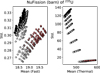 |
Fig. 1 Mean and standard deviation (Std) of the pin-wise neutron production cross section of 235U in the UGd fuel assembly. |
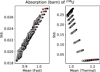 |
Fig. 2 Mean and standard deviation (Std) of the pin-wise absorption cross section of 238U in the UGd fuel assembly. |
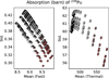 |
Fig. 3 Mean and standard deviation (Std) of the pin-wise absorption cross section of 239 Pu in the MOXfuel assembly. |
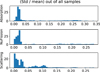 |
Fig. 4 Ratio of standard deviation (Std) over mean values of the pin-wise cross sections of all nuclides in the UGd dataset. |
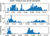 |
Fig. 5 Ratioof standard deviation (Std) over mean values of the pin-wise cross sections of all nuclides in the MOX dataset. |
Mean, Std and maximum values of the fractions fi for neutron absorption of some nuclides from the UGd dataset.
Mean, Std and maximum values of the fractions fi for neutron production of some nuclides from the UGd dataset.
Mean, Std and maximum values of the fractions fi for neutron absorption of some nuclides from the MOX dataset.
Mean, Std and maximum values of the fractions fi for neutron production of some nuclides from the MOX dataset.
6.2 Compression performances
In this section, the HT is applied on the microscopic cross sections arranged according to the matricization M used in Section 3. We study the compression performances for the absorption, for the production (nu-fission) and for the (isotropic) scattering cross sections, which can be used later to setup pin-by-pin core calculations in two-group diffusion theory. Truncation thresholds are varied to ensure sufficient accuracy on reconstructed data as discussed in Section 4.
Homogenized cross sections are prepared for each pin cell by one-eighth fuel assembly calculations, counting K = 45 pin cells, where only 39 cells contain fissile nuclides. The symmetries of the assemblies with reflection boundary condition atall sides are exploited to get faster calculations and to reduce the total storage of output data. The cross sections of the remaining pin cells in the full assembly are obtained in core calculations by the corresponding cell in the eighth of the assembly after unfolding the geometry, and by interpolating with the state parameters at the current local values. Lattice calculations are performed at all physical conditions given by Table 1 ( ). When building the matrices for compression, cross section data are flattened on the group index too, so that the second dimension counts
  elements for absorption and production (
 ), and
  for scattering (
 ). Hence, negative gains are basically prevented; from equation (5) we note that
  . However, this is an optional choice since flattening on the group index can be operated also along the first dimension indexed by k.
After transforming the matrices obtained for each nuclide and reaction type, the truncation is applied by a fixed threshold fraction τ on the total sum of the variances. This truncation threshold relates to the allowed minimum mean squared reconstruction error. This method using a unique value of τ is simpler to implement than using the fractions fi of the macroscopic cross sections introduced in Section 4 to have different threshold values; it already shows very interesting performances. Its behavior changes with the matrix under compression, discarding more or less terms depending on how the pin-wise cross section distributions are correlated. The other method remains of interest for larger data sets, like for instance with compositions of fuel assemblies forming a radial portion of the core that could really demand excessive memory storage.
The spectrum of all covariance matrices shows real eigenvalues differing of many orders of magnitude, that is very large condition numbers. It follows that very small thresholds τ can already discard a large number of components in E. Tables 6 and 7 report the savings μ measured with different threshold values, showing also the mean value and the percentiles at 5%, 50% (median) and 95% of the error distribution in pcm of the multiplication factor k∞. The multiplication factor is calculated by using the same pin-by-pin flux distribution stored in the original dataset and the macroscopic cross sections given by the reconstructed microscopic cross sections, in order to check the neutron balance with the resultant reaction rates and the reference ones from transport. Conforming to the homogenization paradigm, this procedure neglects the changes induced in the flux distribution for using different cross sections in the pins when the assembly sees different neighbors in core calculations. The flux from the dataset is a reference one, because it was computed by the lattice calculation when preparing the original cross sections. The application of an equivalence procedure modifying the homogenized cross sections (like SPH) is of no use in these circumstances because it would conserve by definition the reference reaction rates (and leakage), matching also exactly the reference multiplication factor for any error caused by truncated compression.
The error distribution narrows considerably by tightening the truncation threshold still showing high savings and compression ratios. The pin-wise distributions of rates are smoother in the MOX assembly than in the UGd assembly, and this can be noticed by the fact that higher threshold values can attain higher savings and smaller error on themultiplication factor. Tables 8 and 9 show the largest tails of the relative error distributions in percent on the macroscopic cross sections over all energy groups. Their corresponding 95-th percentiles fall below 0.1% for τ < 10−5. Matrices forscattering cross sections have twice the number of columns and their maximum local errors are higher in general than those of the other reaction types. The use of different truncation thresholds per reaction type is then recommended with separate matrices per nuclide and per reaction type, when the reactor analyst aims primarily atreducing memory occupation. As well, this will yield faster interpolation for fitting fewer compressed coefficients.
Compression performances are even higher when the M -matrices of all the nuclides are vertically stacked by rows for every reaction type, see Tables 10 and 11. In this case the truncation threshold needed to achieve about 1 pcm error on k∞ must be smaller because the condition numbers are even bigger, requesting necessarily double float precision. The numerical transform processes now only three matrices, which are however much larger in size. Hence, matrix multiplication with possibly larger matrices E are also expected with the inverse transformation. However, the HT is so sharp in decorrelating the input data that the new matrices E always stay limited in size for containing very few modes. Tables 12 and 13 show the corresponding largest tails of the relative error distributions in percent on the macroscopic cross sections, with a similar trend to the previouscase.
Errors on the microscopic cross sections present similar trends, and so they are not shown here to limit the printed contents. But they have been carefully checked to avoid any suspicious error compensation. They are studied to check how accurate truncated compressioncan reproduce the original data. The relative errors of the reconstructed microscopic cross sections, estimated by the ratio of the matrix norms of the difference over the reference, as introduced at the end of Section 3, are of O(10−4) when k∞ is accurate up to a few tens of pcm, and decrease further with smaller values of τ. So, we say that the reconstructed values are accurate to about 4 or 5 significant digits.
The original size of the datasets is about 450 MB in memory. Common applications in reactor design can take up to several GBs for a library of a fuel assembly type after considering more state parameters and more specialized nuclides. The acceptable threshold must be selected by testing progressively with smaller values and by measuring the accuracy of the new approximations. Nevertheless, the applications of HT and of its inverse transform take only a small fraction of a second, even on very large matrices. The results presented in this section are obtained with the normalization of the elements of the matrices M by the standard deviation calculated by columns, which improved considerably the global numerical outcome during the computation of these badly conditioned matrices. No negative values were observed when reconstructing the cross sections during this analysis.
There are many possibilities to combine the indices of the dataset (except those in p⃗) to make suitable matrices M for compression. A unique matrix can also be assembled with all the elements of the dataset, provided that enough memory storage is available. This consideration holds for any number of cells dividing the assembly under study, that is also when homogenizing the cross sections over the entire assembly or in one of its quarters. It is clear then that compression can also be used with the existing datasets of ordinary nodal calculations, whose basic unit of the spatial mesh is normally the quarter of assembly.
Error on k∞ in pcm after lossy compression by truncated HT on the UGd dataset with separate matrices M per nuclide and reaction.
Error on k∞ in pcm after lossy compression by truncated HT on the MOX dataset with separate matrices M per nuclide and reaction.
Error on macroscopic cross sections after lossy compression by truncated HT on the UGd dataset with separate matrices M per nuclide and reaction.
Error on macroscopic cross sections after lossy compression by truncated HT on the MOX dataset with separate matrices M per nuclide and reaction.
Error on k∞ in pcm after lossy compression by truncated HT on the UGd dataset with matrices M per reaction type only.
Error on k∞ in pcm after lossy compression by truncated HT on the MOX dataset with matrices M per reaction type only.
Error on macroscopic cross sections after lossy compression by truncated HT on the UGd dataset with matrices M per reaction type only.
Error on macroscopic cross sections after lossy compression by truncated HT on the MOX dataset with matrices M per reaction type only.
6.3 Discussion about interpolation of reconstructed data
The compressed coefficients are stored in the matrix Y by rows, keeping the dependence on the physical state parameters by columns. Each row identifies then the samples of a given coefficient undergoing later interpolation. They show quite regular functions of the state parameters for low frequency modes, but at low burnup values where yet the original cross sections presented steep gradients. This occurs of course for the xenon buildup phenomenon achieving its equilibrium concentration after a few hundreds of MWd/t of exposure at nominal power.
The coefficients and their corresponding modes in the matrix E are sorted in decreasing order of the variances. We observe that the magnitude of the coefficients is decreasing with the higher modes, that is row by row from the first to the last ones, which are associated with high frequency variations. The compressed coefficients appear bounded in finite ranges, and they all verify zero mean caused by the shift with the array m⃗ when building the covariance matrix. The differences in scale among the many cross sections under fit are recovered by the modes, which are never subject to any interpolation process. As an example, Figures 6 and 7 illustrate the behavior of the first and of the fortieth coefficients obtained by compressing the matrix built with the absorption cross sections of all nuclides from the UGd dataset (τ = 10−10 offering the best score in the previous tests). The different colors in the figure represent the behavior of the function along the burnup for fixed values of the other parameters. The outcome for the other cross section types is similar. The compression with this truncation threshold yields 106 coefficients for the UGd dataset and 84 coefficients for the MOX dataset. These numbers yield directly the total number of interpolation to perform in order to evaluate the pin-by-pin homogenized cross sections in 45 pins, for 25 nuclides and in 2 energy groups, thus achieving also a strong saving in time.
The constraint of ensuring positivity that holds when fitting the original cross section functions is no longer needed for the fit of the compressed coefficients. This is an important observation when using polynomials. Since the coefficients of low frequency modes seem mapping smoother functions than for high frequency modes, a low polynomial order shall be enough to yield accurate approximations. Approximations by linear regression could even be proposed for these low frequency coefficients, with the possible use of hard-coded functions to spare fitting coefficients in lookup tables. Whereas higher polynomial orders combined to piecewise representations may be necessary for the coefficients at high frequency. The noticed abrupt change in sign and value of the first coefficient, see Figure 6, can be regularized by setting the xenon concentration in the fuel pins at equilibrium yet at the beginning of the burnup calculation. This quick fix often comes at the cost of using the average xenon concentration in the fuel as a new state parameter. These remarks can help to optimize further the global computational performances since low-order polynomials are faster to evaluate and require the storage of smaller libraries.
It is difficult to compare the applications of the same interpolation problem separately on the set of original cross sections and on the set of their compressed coefficients, because each function shows a different behavior needing a specific approximation method. Microscopic cross sections show very different behaviors over the space described by the state parameters, and general methods, like B-Splines, are recommended to provide accurate approximations [15]. B-splines are smooth functions and have compact support. Provided a suitable knots vector, basis-splines can reproduce simple methods like multi-linear interpolation (B-splines of order 2) or higher-order piece-wise polynomial interpolation [16]. This curve-fitting technique can be proposed for the compressed coefficients too, with a low polynomial order for the low frequency ones. By definition, ordinary interpolation yields the same values of original and reconstructed cross sections at the sampled data sites, which differ only by the truncation error. As a simple test, we performed multi-linear interpolation for the two cases. The comparisons of interpolated cross sections and reconstructed cross sections after interpolation of the compressed coefficients showed differences of the order of the truncation error. Higher interpolation error was noticed with the high frequency coefficients though, but their contribution to the weighted sum of modes was far less important than for the low frequency modes. The search of optimal interpolation schemes with piece-wise polynomials tailored to each compressed coefficient will be addressed in detail with a new research work in the future.
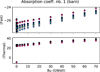 |
Fig. 6 Scatter plot of coefficient 1 along the burnup axis (UGd dataset). |
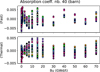 |
Fig. 7 Scatter plot of coefficient 40 along the burnup axis (UGd dataset). |
7 Conclusion
This article presents lossy compression of homogenized pin-by-pin cross sections by the Hotelling transform and threshold truncation. Reconstruction of pin-wise data at any point in the multi-dimensional space built Cartesianly by the state parameters is still achieved by a linear interpolation problem, but fitting straightaway the compressed coefficients. A mathematical demonstration is provided for any kind of linear interpolation problem.
The approach is tested with the datasets given by homogenized cross sections in the pin cells of two PWR fuel assemblies, whose heterogeneous design provides proper use cases. Truncated compression is performed for neutron absorption, scattering and production cross sections, observing high compression ratios also in case of very small truncation thresholds to match narrow tolerances on macroscopic cross sections and on the multiplication factor in the infinite medium. The reconstructed microscopic cross sections were also checked to be accurate up to four significant digits in the most favourable case, being the one with a few large matrices containing all microscopic cross sections of a given reaction type.
Considerable savings in memory are observed with negligible reconstruction errors within the physical tolerance of nuclear data uncertainties and within the numerical tolerance of lattice transport solvers. Specifically, compression ratios higher than 10, corresponding to savings higher than 90%, are noticed in the most conservative cases. As a consequence, important savings in runtime follow for having fewer data to fit by interpolation in multi-physics core calculations relying on pin-wise cross sections. The layout of the matrices being processed is achieved by successive flatten and reshape procedures on multi-dimensional arrays, so that the applied linear algebra methods can also exploit fast vectorized computer operations.
We have considered data sets of homogenized cross sections only in two energy groups because it is the standard option for industrial reactor calculations. A limited number of specialized nuclides was also used to prevent dealing with too large data sets, but still offering a representative use case for core calculations. However, the computational gain is expected to be nearly proportional to the number of nuclides and to the number of energy groups used in the cross section model.
Both test cases presented in this work are about one-eighth assembly calculations. A larger experimental campaign with assemblies showing different design and symmetry types would be necessary to confirm the significant performances achieved by this form of data compression on a general basis. Nonetheless, the compression of homogenized pin-by-pin cross sections by the Hotelling transform with threshold truncation has revealed remarkable results, with consequent important computational gains in runtime when reconstructing function approximations by linear interpolation problems.
Acknowledgements
The author expresses his gratitude to Dr Alberto Previti for the interesting discussions about optimized data storageduring the preparation of the manuscript.
The numerical libraries used in this work are freely distributed for educational purpose. The compression library is available at https://github.com/ndarmage/CmpressLib.git.
The interpolation library is available at https://github.com/ndarmage/pppack.git.
References
- A. Hébert, Applied Reactor Physics (Presses inter Polytechnique, 2009) [Google Scholar]
- R. Sanchez, Assembly homogenization techniques for core calculations, Progr. Nuclear Energy 51, 14–31 (2009) [Google Scholar]
- K.S. Smith, Assembly homogenization techniques for light water reactor analysis, Progr. Nuclear Energy 17, 303–335 (1986) [Google Scholar]
- D. Tomatis, Compression of assembly power form factors for core calculations, Nucl. Sci. Eng. 193, 622–637 (2019) [Google Scholar]
- D. Tomatis, A. Dall’Osso, Compression of 3D pin-by-pin burnup data, Ann. Nucl. Energy 136, 107058 (2020) [Google Scholar]
- A. Yamamoto, T. Ikehara, T. Ito, E. Saji, Benchmark problem suite for reactor physics study of LWR next generation fuels, J. Nucl. Sci. Technol. 39, 900–912 (2002) [Google Scholar]
- H. Sun, Y.Q. Shi, Image and Video Compression for Multimedia Engineering: Fundamentals, Algorithms, and standards (CRC Press, 2008) [Google Scholar]
- G.H. Golub, C.F. Van Loan, in Matrix computations (The John Hopkins University Press, 1996), Vol. 3 [Google Scholar]
- E. Anderson, Z. Bai, C. Bischof, S. Blackford, J. Dongarra, J. Du Croz, A. Greenbaum, S. Hammarling, A. McKenney, D. Sorensen, in LAPACK Users’ Guide (Siam, 1999), Vol. 9 [Google Scholar]
- V.G. Zimin, A.A. Semenov, Building neutron cross-section dependencies for few-group reactor calculations using stepwise regression, Ann. Nucl. Energy 32, 119–136 (2005) [Google Scholar]
- P.M. Bokov, Automated few-group cross-section parameterization based on quasi-regression, Ann. Nucl. Energy 36, 1215–1223 (2009) [Google Scholar]
- D. Botes, P.M. Bokov, Polynomial interpolation of few-group neutron cross sections on sparse grids, Ann. Nucl. Energy 64, 156–168 (2014) [Google Scholar]
- C. De Boor A Practical Guide to Splines (Springer, 1978) [Google Scholar]
- D. Schneider, F. Dolci, F. Gabriel, J.M. Palau, M. Guillo, B. Pothet, P. Archier, K. Ammar, F. Auffret, R. Baron et al., APOLLO3®: CEA/DEN deterministic multi-purpose code for reactor physics analysis, in Proc. Int. Conf. PHYSOR2016, Sun Valley, ID, USA (2016), pp. 2274–2285 [Google Scholar]
- G. Hobson, H.W. Bolloni, K.A. Breith, A. Dall’Osso, R. van Geemert, H. Haase, B. Hartmann, M. Leberig, D. Porsch, B. Pothet et al., ARTEMIS™ Core Simulator: Latest Developments, in Proc. Int. Conf. SNA+MC2013: Joint International Conference on Supercomputing in Nuclear Applications + Monte Carlo, Paris, France (EDP Sciences, 2014), p. 02309 [Google Scholar]
- D. Tomatis, PPPACK, https://github.com/ndarmage/pppack.git (2017) [Google Scholar]
Cite this article as: Daniele Tomatis, A multivariate representation of compressed pin-by-pin cross sections, EPJ Nuclear Sci. Technol. 7, 8 (2021)
All Tables
Mean, Std and maximum values of the fractions fi for neutron absorption of some nuclides from the UGd dataset.
Mean, Std and maximum values of the fractions fi for neutron production of some nuclides from the UGd dataset.
Mean, Std and maximum values of the fractions fi for neutron absorption of some nuclides from the MOX dataset.
Mean, Std and maximum values of the fractions fi for neutron production of some nuclides from the MOX dataset.
Error on k∞ in pcm after lossy compression by truncated HT on the UGd dataset with separate matrices M per nuclide and reaction.
Error on k∞ in pcm after lossy compression by truncated HT on the MOX dataset with separate matrices M per nuclide and reaction.
Error on macroscopic cross sections after lossy compression by truncated HT on the UGd dataset with separate matrices M per nuclide and reaction.
Error on macroscopic cross sections after lossy compression by truncated HT on the MOX dataset with separate matrices M per nuclide and reaction.
Error on k∞ in pcm after lossy compression by truncated HT on the UGd dataset with matrices M per reaction type only.
Error on k∞ in pcm after lossy compression by truncated HT on the MOX dataset with matrices M per reaction type only.
Error on macroscopic cross sections after lossy compression by truncated HT on the UGd dataset with matrices M per reaction type only.
Error on macroscopic cross sections after lossy compression by truncated HT on the MOX dataset with matrices M per reaction type only.
All Figures
|
Fig. 1 Mean and standard deviation (Std) of the pin-wise neutron production cross section of 235U in the UGd fuel assembly. |
| In the text | |
|
Fig. 2 Mean and standard deviation (Std) of the pin-wise absorption cross section of 238U in the UGd fuel assembly. |
| In the text | |
|
Fig. 3 Mean and standard deviation (Std) of the pin-wise absorption cross section of 239 Pu in the MOXfuel assembly. |
| In the text | |
|
Fig. 4 Ratio of standard deviation (Std) over mean values of the pin-wise cross sections of all nuclides in the UGd dataset. |
| In the text | |
|
Fig. 5 Ratioof standard deviation (Std) over mean values of the pin-wise cross sections of all nuclides in the MOX dataset. |
| In the text | |
|
Fig. 6 Scatter plot of coefficient 1 along the burnup axis (UGd dataset). |
| In the text | |
|
Fig. 7 Scatter plot of coefficient 40 along the burnup axis (UGd dataset). |
| In the text | |
Current usage metrics show cumulative count of Article Views (full-text article views including HTML views, PDF and ePub downloads, according to the available data) and Abstracts Views on Vision4Press platform.
Data correspond to usage on the plateform after 2015. The current usage metrics is available 48-96 hours after online publication and is updated daily on week days.
Initial download of the metrics may take a while.