© P. German et al., published by EDP Sciences, 2019

1 Introduction

Molten salt reactor (MSR) designs were originally developed in the mid-1950s at Oak Ridge National Laboratory (ORNL, USA) [1–3]. In MSRs, the nuclear fuel is in liquid form, dissolved in a salt. Salt compositions vary, but are typically based on fluorides or chlorides and include one or more of the following compounds: LiF, NaF, BeF₂, ZrF₄, KF, NaCl, MgCl₂. Diverse variations on that reactor concept were investigated in the 1960s and 1970s, including graphite-moderated thermal-spectrum reactors at ORNL [4, 5] as well as fast-spectrum burner reactors at Argonne National Laboratory [6, 7]. In the early 1970s, MSR research was in competition for U.S. federal funding with sodium-cooled fast reactor systems and the MSR research in the USA dwindled down to low-priority, low-funding efforts over the following decades, while the thermal-spectrum light water-cooled pressurized and boiling water reactors and the sodium-cooled fast reactors became the reference baseline worldwide for thermal and fast spectrum systems, respectively. Nonetheless, electricity-production priorities and safety requirements in the nuclear sector have evolved over the last 50 years and MSRs are now one of the six concepts selected for further investigation in the frame of the Generation-4 International Forum [8]. MSRs have highly promising features in terms of sustainability and safety features. Indeed liquid-fueled MSRs can be designed to have strong negative-only reactivity feedbacks; they operate at atmospheric pressure; they allow for an online removal of gaseous fission products; and they give the possibility to drain the fuel salt in passively cooled and critically-safe tanks in case of emergency. Most fast-spectrum MSRs currently under development are based on pumped-loop designs, where the fuel salt is pumped outside of the primary vessel and transfers heat to a secondary coolant in separate heat exchangers. Examples of fast-spectrum molten salt reactor designs include: the MOlten Salt Actinide Recycler and Transforming (MOSART) project [9], the Molten Salt Fast Reactor (MSFR) concept based on fluoride salt, developed in the EVOL (Evaluation and Viability of Liquid Fuel Fast Reactors) [10–12] and then SAMOFAR (Safety Assessment of the Molten Salt Fast Reactor) [13] programs under the auspices of EURATOM, and the Molten Chloride Fast Reactor (MCFR), currently developed by Terrapower [14]. Loop-type fast-spectrum molten salt reactors present new modeling challenges:

• the fuel is in liquid form, yielding a more complex level of multiphysics coupling than traditional light water reactors (e.g., velocity fields needed to assess space/time location of fuel and delayed neutron precursors);

• turbulent fuel-salt flow, leading to a large impact of turbulence modeling (thermal flow mixing in the core, effects of nozzle inlets,... [15]);

• presence of gas bubbles in the salt, leading to compressibility and reactivity effects;

• high solidification temperature of the salt, requiring the modeling of solidification/melting zones (wall solidification, frozen drain functionality, see [15]);

• high operating temperature in the salt, necessitating the study of thermal radiation heat transfer.

The modeling challenges in fast-spectrum MSRs largely prohibit the use of simulation packages developed and tailored specifically for Light WaterReactors (LWRs). For instance, the Virtual Environment for Reactor Applications (VERA), developed as part of the Consortium for Advanced Simulation of Light water reactors (CASL) is being leveraged for MSR modeling but is only at an early stage of development for MSR and mostly focused on thermal-spectrum reactors, where salt flows mostly uni-directionally in graphite channels [16, 17]. Hence, high-fidelity models, based on first-principle physics, become the only available tool to gain understanding of the significance of foreseeable phenomena unique to molten salt and circulating fuel systems. Driven by the need for high-fidelity computational fluid dynamics (CFD), many research teams developing fast-spectrum MSRs rely on the open-source OpenFOAM CFD platform, either directly [18, 19] or embedded in reactor physics packages such as GeN-Foam (Generalized Nuclear Foam) [20, 21].

However, the simulation of such complex systems requires the solution of coupled partial differential equations, which can be computationally expensive to obtain. Model-order reduction comprises a set of empirical and mathematical techniques that can be used for lowering the computational complexity of the Full-Order Models (FOM) by creating Reduced-Order Models (ROM) that sacrifice a modest amount of accuracy for large gains in compute time. An effective mathematical technique for model-order reduction is the Reduced Basis (RB) method, which is based on the assumption that the solution of a complex model lives in a relatively small subspace. When parametric studies are to be performed, one should expand that subspace to account for solution variability. One manner by which such a subspace is “discovered” is through multiple full-order solutions, with adequate sampling of the parameter (input) space. This is known as the method of snapshots. The information contained in these snapshots isthen extracted by means of Proper Orthogonal Decomposition (POD) [22, 23] (e.g., via correlation matrix or singular value decompositions). The FOM is then Galerkin-projected on the obtained basis functions to yield the ROM. In this work, a POD-based ROM is created for parametrized multiphysics computations on the Dopplerfeedback effect in the Molten Salt Fast Reactor (MSFR) [24, 25]. In this technique, the FOM is projected onto an appropriate subspace obtained via a POD of solutions determined by exercising the FOM itself. In other words, snapshots are taken at different states of the FOM and a POD is used to build a suitable basis for projection-based reduction. In the nuclear engineering community, applications of POD -based ROMs can be noted in reactor kinetics problems [26, 27], fixed source, steady state neutral particle transport applications [28]. An approach for POD-ROM of eigenvalue problems connected to reactor physics has already been developed in [29–33].

However, the utilization of POD-based ROM for multiphysics applications can be challenging because the operators in the full-order models often do not have an affine decomposition, meaning that the ROMs involve costly, full-order operations, possibly yielding negligible savings in computation time. A method for the reduced-order modeling of multiphysics problems in nuclear engineering has also been derived in [30]. The approach described in the present work serves as an alternative. Instead of assuming an overall linear temperature dependence for the cross sections, here we opt for a hyper-reduction technique, namely, the Discrete Empirical Interpolation Method (DEIM) [34]. This allows the handling of an arbitrary, non-linear temperature dependence of the cross sections (in our case, in the logarithm of temperature). Our approach is exemplified using a liquid nuclear fuel system, more specifically, for a simplified 2D model of the Molten Salt Fast Reactor. The methodology has been integrated into GeN-Foam. For different applications of DEIM in other fields of engineering, we refer the reader to [35–37].

The rest of the paper is organized as follows. In Section 2, projection-based model order reduction is reviewed, first for linear systems, then for nonlinear systems, such as the ones encountered in multiphysics applications. In Section 3, a full-order simulation model is provided for a fast-spectrum molten salt reactor and its associated reduced-order model is derived. Section 4 describes the chosen MSFR computational model and its parametric input space. Results comparing the FOM and ROM models are provided in Section 5. We conclude and propose future work in Section 6.

2 Model order reduction: background

In this section, we review some of the basics of projection-based model-order reduction. For brevity of the exposition, the reduced basis will always be sought through a POD decomposition and the reduced system will always be obtained using Galerkin projection. We refer the reader to [38, 39] for other reduced basis approaches and to [40] for Petrov-Galerkin projection-based ROM.

2.1 Model order reduction for linear systems

First, we consider a linear parameterized steady-state FOM. After discretization, the FOM can be written as $$A(\mu )x(\mu )=b(\mu ),$$(1)

where $A(\mu )\in {ℝ}^{N\times N}$ is the discretized linear operator (a possibly large system of dimension N), $x(\mu )\in {ℝ}^N$ is the solution vector and the parametric dependence of the model is denoted by the d-dimensional input parameter vector $\mu ={[{\mu }_1,\dots ,{\mu }_d]}^T$. In order to discover the lower dimension manifold in which the parametric solutions can be adequately represented,the FOM is exercised for a certain number of realizations of the input parameter vector μ_i, with 1 ≤ i ≤ N_S and N_S denoting the number of snapshots. Letting $S=[x({\mu }_1),\dots ,x({\mu }_{N_S})]\in {ℝ}^{N\times N_S}$ denote the snapshot matrix, we perform a POD on S, which constructs an orthonormal basis $V=[v_1,\dots ,v_r]\in {ℝ}^{N\times r}$ where only the r most dominant modes are retained. A computationally effective manner to do this consists in generating the correlation matrix $\mathcal{Q}$ of the snapshots as $$\mathcal{Q}=S^{T}S.$$(2)

Then, the eigenvalue decomposition of the correlation matrix is obtained $$\mathcal{Q}=\mathcal{W}\Lambda {\mathcal{W}}^T,$$(3)

where $\mathcal{W}=[w_1,\dots ,w_{N_s}]$ is the matrix of eigenvectors and Λ is a diagonal matrix containing the Λ_i eigenvalues. The orthonormal basis vectors in V can then be constructed using the snapshots by $$v_j=\frac{1}{\sqrt{{\Lambda }_i}}{\displaystyle \sum _{i=1}^{N_s}x}({\mu }_i)w_{j,i}.$$(4)

Once this offline stage has been completed, the reduced order model is obtained by projection of the full order system: $$A_r(\mu )x_r(\mu )=b_r(\mu ),$$(5)

with the reduced linear operator $A_r(\mu )=V^{T}A(\mu )V\in {ℝ}^{r\times r}$, reduced right-hand side $b_r(\mu )=V^{T}b(\mu )\in {ℝ}^r$, and the reduced state vector $x_r(\mu )\in {ℝ}^n$. This linear system of size r ≪ N, is solved for x_r, which are the coefficients of the full-order solution in the basis V. Hence, the full-order solution is reconstructed as $$x\approx {\sum }_{i=1}^r{v}_i{x}_{r,i}=V{x}_r.$$(6)

For additional information, we refer the reader to [41, 42].

2.2 Model order reduction for nonlinear systems

Next, we consider a nonlinear full-order model (FOM) which, after discretization, can be written as $$A(\mu )x(\mu )+F(x(\mu ),\mu )=b,$$(7)

where a nonlinear vector-valued function has been added, $F(x(\mu ),\mu )\in {ℝ}^N$. Henceforth, for the sake of easier readability, the dependence of the operators on μ is only assumed and not shown explicitly. If one carries out the procedures described in Section 2.1, the resulting nonlinear reduced-order model is $$A_r{x}_r(\mu )+V^{T}F(V{x}_r(\mu ))=b_r.$$(8)

Even though this equation is expressed in terms of the vector of reduced unknowns, x_r, solving it requires evaluating the full-order nonlinear vector-valued function, of size N ≫ r. This can be computational very expensive, often resulting in limited CPU time savings when solving the reduced order model, compared to the original full-order model. To remedy this, the Discrete Empirical Interpolation Method (DEIM) [34] is used in order to approximate F in a low-dimensional space by sampling it at only m ≪ N components. Hence, during the offline stage, a second matrix of snapshots is collected for the nonlinear function values, $S_F=[F(x({\mu }_1)),\dots ,F(x({\mu }_{N_S}))]\in {ℝ}^{N\times N_S}$. Similarly to the method described in equations (2)–(4), the POD of S_F is computed and m of the basis functions for the nonlinear vector-valued function are retained to subsequently interpolate F: $[u_1,\dots ,u_m]=U\in {ℝ}^{N\times m}$. DEIM also selects m distinct interpolation points p₁, …, p_m ∈ [1, N] in order to assemble the DEIM interpolation point matrix $P=[e_{p_1},\dots ,e_{p_m}]\in {ℝ}^{N\times m}$, where e_i is the ith canonical unit vector. Finally, the DEIM interpolant of F is $$U{(P^{T}U)}^{-1}{P}^{T}F(x(\mu )),$$

and the resulting nonlinear reduced-order model system is $$A_r{x}_r(\mu )+V^{T}U{(P^{T}U)}^{-1}{P}^{T}F(V{x}_r(\mu ))=b_r.$$(9)

Several remarks are in order:

• $V^{T}U{(P^{T}U)}^{-1}\in {ℝ}^{r\times m}$ is a small matrix that can be pre-computed once for all;

• P^T F extracts only a few (actually m, with m ≪ N) components of F that need to be evaluated. This is a large savings afforded by the use of the DEIM. Because discretization of partial differential equations usually results in local connectivity between an unknown and its neighbors, evaluating P^T F(V x(μ)) is therefore computationally inexpensive when m ≪ N.

For additional information on DEIM, we refer the reader to [34, 43].

3 Governing laws

In this section, we select mathematical models (partial differential equations) that will be used as FOM and derive their reduced-order counterparts. These models are said to be parametric in the sense that certain parameters are uncertain in the governing equations and will be sampled from appropriate probability density functions. In this work, the following parameter are assumed uncertain: the total reactor power (P_th), the heat exchange coefficient in the heat sink, i.e., in the heat exchanger (α_ext), the ultimate heat sink temperature (T_ext), and the volumetric area of the heat sink (A_V). The vector containing all the uncertain parameters will be denoted by $\mu ={({\alpha }_{\text{ext}},A_V,T_{\text{ext}},P_{\text{th}})}^T$.

The mathematical models are selected to be representative of a simplified molten salt reactor design. The molten salt reactor application is discussed in a later section.

3.1 Full-Order Model (FOM)

In order to represent the physics of a MSFR, we define a multiphysics model comprising of

• neutronics: six-group k-eigenvalue diffusion theory, with delayed neutron precursor balance equation with a drift (advection) term, and

• thermal-hydraulics: here, we only consider an energy balance equation, with a given (but spatial varying) flow field computed using nominal values of the uncertain parameters. For the types of parametric modifications employed here, the effect of flow perturbations should be small. For the reduced-order modeling for turbulent flows, we refer the reader to [44, 45].

The cross sections in the neutronics models are temperature-dependent. The multi-group diffusion k-eigenvalue problem [46] can be described asa coupled partial differential equation system expressing the balance of neutrons in each energy bin as $$\begin{array}{lll}\hfill & \hfill & -\nabla \cdot (D_g\nabla {\Phi }_g)+{\Sigma }_{r,g}{\Phi }_g=\frac{(1-\beta ){\chi }_{p,g}}{k}{\sum }_{g^{\prime }=1}^G\nu {\Sigma }_{f,g^{\prime }}{\Phi }_{g^{\prime }}\hfill \\ \hfill & \hfill & +{\chi }_{d,g}{\sum }_{i=z}^I{\lambda }_z{C}_z+{\sum }_{g^{\prime }\ne g}^G{\Sigma }_{g^{\prime }\to g}{\Phi }_{g^{\prime }},\hfill \end{array}$$(10)

where G denotes the number of energy groups, I the number of delayed neutron precursor groups, Φ_g is the neutron scalar flux, D_g is the diffusion coefficient, Σ_r,g is the macroscopic removal cross-section and νΣ_f,g is the total fission neutron yield times the macroscopic fission cross-section in energy group g. Furthermore, ${\Sigma }_{g^{\prime }\to g}$ is the macroscopic scattering cross-section from group g′ to g, χ_p,g and χ_d,g describe the fraction of prompt and delayed neutrons released in group g, while β is the effective delayed neutron yield. Moreover, λ_z denotes the decay constant corresponding to the delayed neutron precursor concentration C_z of group precursor group z. The problem is supplemented with boundary conditions: reflective boundary conditions $(\nabla {\Phi }_g\cdot n=0,g=1,\dots ,G)$ are applied on the symmetry planes and zero-incoming current boundaries are applied on the other boundaries ($-D_g\nabla {\Phi }_g\cdot n=\frac{1}{2}{\Phi }_g$, g = 1, …, G). These equations are coupled with the steady-state balance equations for the delayed neutron precursors, commonly expressed as $$\nabla \cdot (u{C}_z)-\nabla \cdot ({\alpha }_{\text{eff}}\nabla C_z)=\frac{{\beta }_z}{k}{\sum }_{g=1}^G\nu {\Sigma }_{f,g}{\Phi }_g-{\lambda }_z{C}_z,$$(11)

where $u$ is a precomputed (stationary) velocity field, β_z is the delayed neutron yield for precursor group z and α_eff is an effective diffusion coefficient that takes into account the effects of turbulent mixing as well. For simplicity, zero gradient boundary conditions ($\nabla C_z\cdot n=0$ for z = 1, …, I) are used for each of the precursor equations on every wall. We stress that $u$ is not uniform, but taken from a CFD simulation using the nominal values of the uncertain parameters (the RANS continuity and momentum equations were solved using k−ɛ model for turbulence [21]). Thus, $u$ and α_eff are known fields during the generation of the reduced operators. We leave model-order reduction of turbulent hydrodynamics for subsequent work. The multigroup neutron fluxes are normalized using the group-wise power cross section Σ_p,g to ensure a certain total reactor power, P_th: $${\displaystyle {\int }_{\text{domain}}{d}^3}r{\sum }_{g=1}^G{\Sigma }_{p,g}(r){\Phi }_g(r)=P_{\text{th}}.$$(12)

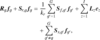
The cross sections are assumed to be temperature-dependent. For fast spectrum reactors, as shown in [47], a logarithmic interpolation between pre-computed data-bases (for example at 900 K and 1200 K) of the group constants yields good results: $$\begin{array}{lll}\Sigma (T)\hfill & =\hfill & {\Sigma }_{900}+\frac{{\Sigma }_{1200}-{\Sigma }_{900}}{\log \left(\frac{1200}{900}\right)}\log \left(\frac{T}{900}\right)\hfill \\ \hfill & =\hfill & {\Sigma }^{\text{const}}+{\Sigma }^{\text{var}}\log (T).\hfill \end{array}$$(13)

where T denotes the temperature field.

Finally, to be able to account for the temperature feedback, the following energy balance equation is solved: $$\nabla \cdot (u\rho c_{p}T)=\nabla \cdot (k_T\nabla T)-\alpha A_V(T-T_{\text{ext}})+{\sum }_{g=1}^G{\Sigma }_{p,g}{\Phi }_g,$$(14)

where ρ is the density, c_p is the heat capacity, k_T the effective thermal conductivity of the fluid, while α is the heat transfer coefficient and A_V is the volumetric area of the heat sink. All of the parameters in the equation above are assumed to be constant. Furthermore, the heat transfer coefficient α is computed as the harmonic mean of two coefficients, one that characterizes the heat transfer between the salt and the structure of the heat exchanger (α_salt) and a second describing the heat flow between the heat exchanger and the external heat sink (α_ext). For simplicity, zero gradient boundary conditions $(\nabla T\cdot n=0)$ are used for every surface in the model. The iteration scheme used for the solution of the coupled problem is discussed in details in [21]. α_ext, A_V and T_ext are assumed uncertain; hence this model is parametric in those input parameters.

3.2 Reduced-Order Model (ROM)

The ROMs are constructed by physics-wise (equation-wise) projection of the FOM equations onto suitable reduced bases obtained applying POD to the solution snapshots. During the offline phase, the solution fields are collected into corresponding snapshot matrices and a Proper Orthogonal Decomposition is carried out for each snapshot matrix separately. This segregated approach has been proven to be effective for k-eigenvalue multigroup problems [33]. The approximate solutions in the reduced spaces can be written as 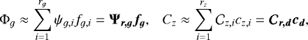$${\Phi }_g\approx {\displaystyle \sum _{i=1}^{r_g}{\psi }_{g,i}}{f}_{g,i}={\Psi }_{r,g}{f}_g, C_z\approx {\displaystyle \sum _{i=1}^{r_z}{\mathcal{C}}_{z,i}}{c}_{z,i}={\mathcal{C}}_{r,d}{c}_d,$$(15) $$T\approx {\displaystyle \sum _{i=1}^{r_T}{\tau }_i}{t}_i={\mathcal{T}}_{r}t, \log (T)\approx {\displaystyle \sum _{i=1}^{r_l}{\mathcal{L}}_i}{l}_i={\mathcal{L}}_{r}l$$(16)

where ψ_g,i is the ith basis vector of the subspace selected for the neutron flux in group g, ${\mathcal{C}}_{z,i}$ is the ith basis vector for the precursor group z, τ_i denotes the basis vector of temperature and ${\mathcal{L}}_i$ is the ith basis vector of the logarithmic temperature. Moreover, f_g, c_d, t and l vectors contain the coordinates of the approximated flux in group g, approximated precursor concentration in group d, approximated temperature and logarithmic temperature within their corresponding reduced spaces. 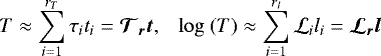Using these, the ROMs for the multi-group diffusion equations can be described as $$\begin{array}{lll}{R}_g{f}_g+S_{r,g}{f}_g\hfill & =\hfill & \frac{1}{k_r}{\sum }_{g^{\prime }=1}^G{S}_{f,g^{\prime }}{f}_{g^{\prime }}+{\sum }_{z=1}^I{L}_z{c}_z\hfill \\ \hfill & \hfill & +{\sum }_{g^{\prime }\ne g}^G{S}_{s,g^{\prime }}{f}_{g^{\prime }},\hfill \end{array}$$(17)

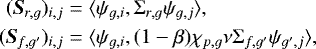
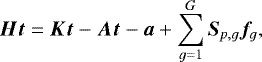
where k_r is the largest eigenvalue of the reduced system and the reduced operators are computed using the approximation mentioned in equation (15) together with a Galerkin projection onto the corresponding subspace. Thus, the elements of the reduced diffusion operator can be expressed as $${(R_g)}_{i,j}=\langle {\psi }_{g,i},-\nabla \cdot (D_g\nabla {\psi }_{g,j})\rangle ,$$(18)

where ⟨ ⋅ ⟩ denotes the volumetric integral of the given scalar fields that can be carried out numerically. Even though it is not shown explicitly, this reduced operator takes into account the boundary conditions imposed on the scalar flux by incorporating a 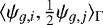${\langle {\psi }_{g,i},\frac{1}{2}{\psi }_{g,j}\rangle }_{\Gamma }$ term (in case of vacuum boundary) for every boundary face Γ of the computational domain. Again, it must be mentioned, that D_g depends on the approximate logarithmic temperature (see Eq. (16)). By translating this linear dependence into the ROM, the expressions of the reduced operators become slightly more convoluted and can be written as $$\begin{array}{lll}{(R_g)}_{i,j}\hfill & \hfill & =\langle {\psi }_{g,i},-\nabla \cdot (D_g^{\text{const}}\nabla {\psi }_{g,j})\rangle \hfill \\ \hfill & \hfill & +{\displaystyle \sum _{k=1}^{r_l}\langle {\psi }_{g,i},-\nabla \cdot (}{D}_g^{\text{var}}{\mathcal{L}}_k\nabla {\psi }_{g,j})\rangle l_k,\hfill \end{array}$$(19)

where the values of $D_g^{\text{const}}$ and $D_g^{\text{var}}$ can be determined using equation (13) and the coefficients of the logarithmic temperature (l_i) are computed using the coefficients of the temperature (t_i) through the Discrete Empirical Interpolation Method, described in Section 2.2 in detail, as follows: $$l={(P^T{L}_r)}^{-1}\log (P^T{\mathcal{T}}_{r}t).$$

It should be noted that, in this case, it is enough the carry out the DEIM in terms of the logarithm of the temperature due to the fact that the nonlinearity in the model is caused by the temperature-dependence of the cross sections, and the non-linear function involves the logarithm of the temperature. As noted in the previous Section, we recall that the reduced operator can be precomputed in a tensor form and every time the operator has to be reconstructed due to the changing temperature field, it only requires the summation of reduced matrices making the coupling of the reduced models extremely efficient. The same treatment is applied to the other reduced operators containing cross-sections, even though in the following definitions it is not shown explicitly. The additional reduced operators in equation (17) are computed as $$\begin{array}{lll}{(S_{r,g})}_{i,j}\hfill & =\hfill & \langle {\psi }_{g,i},{\Sigma }_{r,g}{\psi }_{g,j}\rangle ,\hfill \\ {(S_{f,g^{\prime }})}_{i,j}\hfill & =\hfill & \langle {\psi }_{g,i},(1-\beta ){\chi }_{p,g}\nu {\Sigma }_{f,g^{\prime }}{\psi }_{g^{\prime },j}\rangle ,\hfill \end{array}$$(20) $$\begin{array}{lll}{(L_z)}_{i,j}\hfill & =\hfill & \langle {\psi }_{g,i},{\chi }_{d,g}{\lambda }_z{\mathcal{C}}_{z,j}\rangle ,\hfill \\ {(S_{s,g^{\prime }})}_{i,j}\hfill & =\hfill & \langle {\psi }_{g,i},{\Sigma }_{g^{\prime }\to g}{\psi }_{g^{\prime },j}\rangle .\hfill \end{array}$$(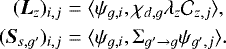21)

One can notice that these reduced matrices may be rectangular depending on the number of POD modes used for the different reduced bases. Similarly, the reduced form of the precursor equations can be expressed as 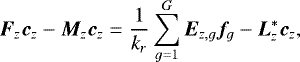$$F_z{c}_z-M_z{c}_z=\frac{1}{k_r}{\sum }_{g=1}^G{E}_{z,g}{f}_g-L_z^{*}{c}_z,$$(22)

where the entries of the reduced operators are computed as $$\begin{array}{lll}\hfill & \hfill & {(F_z)}_{i,j}=\langle {\mathcal{C}}_{z,i},\nabla \cdot (u{\mathcal{C}}_{z,j})\rangle ,\hfill \\ \hfill & \hfill & {(M_z)}_{i,j}=\langle {\mathcal{C}}_{z,i},\nabla \cdot ({\alpha }_{\text{eff}}\nabla {\mathcal{C}}_{z,i})\rangle ,\hfill \end{array}$$(23) $$\begin{array}{lll}\hfill & \hfill & {(E_{z,g})}_{i,j}=\langle {\mathcal{C}}_{z,i},{\beta }_z\nu {\Sigma }_{f,g}{\psi }_{g,j}\rangle ,\hfill \\ \hfill & \hfill & {(L^{*}{}_z)}_{i,j}=\langle {\mathcal{C}}_{z,i},{\lambda }_z{\mathcal{C}}_{z,j}\rangle .\hfill \end{array}$$(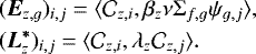24)

As a last step, the reduction of the energy equation is carried out as $$Ht=Kt-At-a+{\sum }_{g=1}^G{S}_{p,g}{f}_g,$$(25)

where the entries of the reduced matrices and sink vector are given by $${(H)}_{i,j}=\langle {\tau }_i,\nabla \cdot (u\rho c_p{\tau }_j)\rangle {(K)}_{i,j}=\langle {\tau }_i,\nabla \cdot (k_T\nabla {\tau }_j)\rangle$$(26) $${(A)}_{i,j}=\langle {\tau }_i,-\alpha A_V{\tau }_j\rangle {(a)}_i=\langle {\tau }_i,\alpha A_V{T}_{\text{ext}}\rangle$$(27) $${(S_{p,g})}_{i,j}=\langle {\tau }_i,{\Sigma }_{p,g}{\psi }_{g,j}\rangle .$$(28)

Finally, we note that the elements of input parameter vector $\mu ={({\alpha }_{\text{ext}},A_V,T_{\text{ext}},P_{\text{th}})}^T$ are simply factors in the reduced order equations as well, thus the reconstruction of the reduced matrices is not necessary for repeating simulations with the ROM. For the solution of the coupled problem, the standard GeN-Foam iteration scheme is used which is discussed in paper [48] in detail. The same iterative scheme is used to solve both the FOM and the ROM models. To compare the solutions of the ROM with those of the FOM we use the following two error indicators: $$\Delta k=|k-k_r|,$$(29)

that describes the absolute difference between the largest eigenvalue of FOM and the ROM, and $$e_{\zeta }=\frac{\left|\right|{\zeta }_{\text{FOM}}-{\zeta }_{\text{ROM}}|{|}_{L^2}}{\left|\right|{\zeta }_{\text{FOM}}|{|}_{L^2}}$$(30)

that gives the relative L² error in the field variables, where ζ can be Φ_g (g = 1, …, G), C_z (z = 1, …, I) or T.

4 MSFR computational model

A 2D axisymmetric model of the MSFR has been created using the available information in [18, 48, 49]. The dimensions of the geometry are provided in Figure 1 together with the pre-computed velocity field. The velocity field has been obtained by a standalone steady state solve of the incompressible porous Navier-Stokes equations with k-ɛ turbulence model [21]. The heat exchanger (HX) is modeled as a porous medium responsible for flow resistance and heat sink, while the pump (P) is modeled as a simple volumetric momentum source. For more information about the semi-empirical expressions used to compute the parameters of the flow resistance and heat sink, the reader may refer to [21].

The mesh used for the computations has been created using SALOME [50] and contains 11,064 cells. For the neutronics computations, six energy and eight precursor groups are used, meaning that the full-order model has 165,960 degrees of freedom. The corresponding group constants are generated using Serpent 2 Monte Carlo Transport code [51] for two salt temperatures, 900 K and 1200 K. The bounds of the used energy group structure are presented in Table 1.

Altogether 20 parameter vectors are sampled for snapshot generation using the Improved Distributed Latin Hypercube Sampling (IHS) method [53]. The uncertain parameters in these vectors are varied in a ± 20% interval around their mean values $\overline{\mu }=({10}^5$ W m⁻²K, 100 m² m⁻³, 900 K, 1440 MW_th). Using these snapshots, altogether 16 reduced spaces are created using POD. One for the neutron flux in each energy group, one for the precursor concentration in each group, one for the temperature and one for the logarithmic temperature. The decay in the eigenvalue of the correlation matrices (defined in Eq. (2)) are presented in Figure 2; the eigenvalues are normalized to their largest one. It is visible that for all field variables, the eigenvalues decay rapidly, suggesting that only a few modes are enough to approximate the full-order solution. It can also be observed that, as the half-life of the precursor group decreases (from group 1 to 8), the decay in the eigenvalues of the corresponding correlation matrices is slower.

The dimensions of the reduced spaces for the different solution fields are summarized in Table 2. These numbers are acquired using a strategy based on the energy-retention limit defined as $$\frac{{\displaystyle \sum _i^{r_i}{\lambda }_i}}{{\displaystyle \sum _i^{N_s}{\lambda }_i}}<1-{\varepsilon }_{\text{lim}},$$

where λ_i are the eigenvalues of the correlation matrix built using the snapshots of a selected field, r is the number of POD modes retained for this field and (1 − ɛ_lim) is the energy-retention limit. This characterizes the error in the reconstruction of the snapshots originating from discarding the rest of the POD modes (r + 1, …, N_s). When ɛ_lim = 0, all of the POD modes are used, hence the snapshots can be reconstructed exactly. In this work, ɛ_lim = 10⁻⁷ was used.

The relatively low dimensions can be explained by the fact that all the uncertain parameters appear in the thermal balance equation and changing them does not influence the distributions of flux and temperature fields considerably. This also means that the 165,960 degrees of freedom in the FOM can be reduced to 27 unknowns in the ROM.

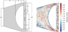Fig. 1 The geometry and flow field used for the snapshot generation with the FOM. Dimensions are shown in mm. (P – Pump, HX – Heat Exchanger).

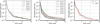Fig. 2 The decay in the eigenvalues of correlation matrices for the neutron flux (left), precursor concentration (middle) and temperature (right).

5 Results

After building the reduced-order model, a new realization of the input parameter vector, μ^* = (9.3 × 10⁴ W m⁻²K, 111.1 m² m⁻³, 833.3 K, 1320 MW_th) is selected and simulations are performed with both the ROM and the FOM in order to test the accuracy and efficacy of the ROM. We stress that μ^* was not included in the training set. Figure 3 shows the reconstructed scalar flux in energy group one from the ROM together with its absolute deviation from the full order solution. It is visible that the maximum error is more than three orders of magnitude lower than the maximum value of the full order solution.

Figure 4 compares the precursor concentration in precursor group eight. Again, it is visible that the maximum absolute deviation is approximately three orders of magnitude lower than the maximum of the original solution. Figure 5 shows the reconstructed temperature profile of the ROM with its relative deviation from the FOM. Again, the maximum relative error is slightly above 1%. Furthermore, the deviation between the effective multiplication factors coming from the ROM and FOM was 8.5 pcm, which is also satisfactory. It is worth noting that loosening the energy-retention limit to 10⁻⁶ resulted a 77.6 pcm difference in the eigenvalues, while tightening it to 10⁻⁸ gave 22.3 pcm due to the inclusion of a third POD mode for the logarithmic temperature that decreased the accuracy in the temperaturecoefficients. By further increasing the energy-retention limit, we observed no further change from the 22 pcm difference level.

Furthermore, the relative L² errors in thefield variables, defined at equation (30), are summarized in Table 3. It can be observed that none of the fields have a relative L² error above 1%. The speed-up factor for the solution of the problem was 1550 for this specific example.

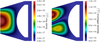Fig. 3 The reduced order solution for the scalar flux in energy group one together with its absolute deviation from the full order solution.

Fig. 4 The reduced order solution for the precursor concentration in group eight together with its absolute deviation from the full order solution.

Fig. 5 The reduced order solution for the temperature together with its absolute deviation from the full order solution.

6 Conclusions

An efficient way of coupling parametrized neutronics and energy equations has been developed for POD-based ROMs. It utilizes the group-wise projection of the multi-group diffusion equations, including the precursor balance equations, and the enthalpy equation in moving fuel systems. In the current state of the development, the velocity equations are not solved; a constant velocity field is assumed. The non-linear temperature dependence of the group constants is handled using DEIM. To demonstrate the viability of the method, it has been implemented in OpenFOAM based multiphysics solver, GeN-Foam. Moreover, a ROM has been created for the MSFR and the corresponding reduced spaces have been generated by exercising a simplified 2D axisymmetric FOM. The limited number of parameters and the underlying physics resulted in reduced spaces with dimensions between 1-3. A test has been performed with four uncertain parameters in the energy equation and the results of the ROM have been compared to those of the FOM. A good agreement is observed both in terms of thesolution vectors and the effective multiplication factors. The experienced speed up factor was above 1,500.

Acknowledgements

This material is based upon work supported under an NEUP-IRP Award of the U.S. Department of Energy, Office of Nuclear Energy (contract reference DE-NE0008651).

References

All Tables

All Figures

	Fig. 1 The geometry and flow field used for the snapshot generation with the FOM. Dimensions are shown in mm. (P – Pump, HX – Heat Exchanger).
In the text

	Fig. 2 The decay in the eigenvalues of correlation matrices for the neutron flux (left), precursor concentration (middle) and temperature (right).
In the text

	Fig. 3 The reduced order solution for the scalar flux in energy group one together with its absolute deviation from the full order solution.
In the text

	Fig. 4 The reduced order solution for the precursor concentration in group eight together with its absolute deviation from the full order solution.
In the text

	Fig. 5 The reduced order solution for the temperature together with its absolute deviation from the full order solution.
In the text

References

- M.W. Rosenthal, P.R. Kasten, R.B. Briggs, Molten-salt Reactors – history, status, and potential, Nucl. Appl. Technol. 8, 107 (1970) [CrossRef] [Google Scholar]
- D. LeBlanc, Molten salt reactors: a new beginning for an old idea, Nucl. Eng. Des. 240, 1644 (2010) [CrossRef] [Google Scholar]
- H.G. MacPherson, The molten salt reactor adventure, Nucl. Sci. Eng. 90, 374 (1985) [CrossRef] [Google Scholar]
- R. Robertson, MSRE design and operations report. Part I. Description of reactor design, Tech. Rep. ORNL-TM-728, 1965, DOI:10.2172/4654707 [CrossRef] [Google Scholar]
- M.W. Rosentahl, The development status of molten-salt breeder reactors, Tech. Rep. ORNL-4812, 1972 [Google Scholar]
- L.G. Alexander, Molten-Salt Fast Reactors, Tech. Rep. ANL-6792, 1963 [Google Scholar]
- D. Holcomb, et al., Fast Spectrum Molten Salt Reactor Options, Tech. Rep. ORNL/TM-2011/105, 2011 [Google Scholar]
- The Generation IV International Forum (GIF), https://www.gen-4.org/gif/, Accessed: 04-10-2019 [Google Scholar]
- V. Ignatiev, O. Feynberg, I. Gnidoi, A. Merzlyakov, A. Surenkov, V. Uglov, A. Zagnitko, V. Subbotin, I. Sannikov, A. Toropov, et al., Molten salt actinide recycler and transforming system without and with Th-U support: fuel cycle flexibility and key material properties, Ann. Nucl. Energy 64, 408 (2014) [CrossRef] [Google Scholar]
- L. Mathieu, D. Heuer, E. Merle-Lucotte, R. Brissot, C. Le Brun, E. Liatard, J.-M. Loiseaux, O. Méplan, A.Nuttin, D. Lecarpentier, Possible configurations for the thorium molten salt reactor and advantages of the fast nonmoderated version, Nucl. Sci. Eng. 161, 78 (2009) [CrossRef] [Google Scholar]
- D. Heuer, E. Merle-Lucotte, M. Allibert, M. Brovchenko, V. Ghetta, P. Rubiolo, Towards the thorium fuel cycle with molten salt fast reactors, Ann. Nucl. Energy 64, 421 (2014) [CrossRef] [Google Scholar]
- EVOL (Project no249696) Final Reportr, https://cordis.europa.eu/docs/results/249/249696/final1-final-report-f.pdf, Accessed: 04-10-2019 [Google Scholar]
- SAMOFAR (Safety Assessment of the Molten Salt Fast Reactor), http://samofar.eu/, Accessed: 04-10-2019 [Google Scholar]
- MCFR Solutions: Nuclear Innovation for New Options in American Industry, https://terrapower.com/technologies/mcfr, Accessed: 04-10-2019 [Google Scholar]
- M. Tano-Retamales, Modélisation multi-physique multi-échelle de caloporteurs sels fondus et validation expérimentale, Ph.D. thesis, Université Grenoble-Alpes, 2018 [Google Scholar]
- B.S. Collins, C.A. Gentry, A.J. Wysocki, R.K. Salko, Molten salt reactor simulations using MPACT-CTF, Tech. rep., Oak Ridge National Lab.(ORNL), Oak Ridge, TN (United States), 2017 [Google Scholar]
- C.A. Gentry, B.R. Betzler, B.S. Collins, Initial Benchmarking of ChemTriton and MPACT MSR Modeling Capabilities, Tech. rep., Oak Ridge National Laboratory (ORNL), Oak Ridge, TN (United States), 2017 [Google Scholar]
- M. Aufiero, A. Cammi, O. Geoffroy, M. Losa, L. Luzzi, M.E. Ricotti, H. Rouch, Development of an OpenFOAM model for the Molten Salt Fast Reactor transient analysis, Chem. Eng. Sci. 111, 390 (2014) [CrossRef] [Google Scholar]
- A. Laureau, D. Heuer, E. Merle-Lucotte, P. Rubiolo, M. Allibert, M. Aufiero, Transient coupled calculations of the Molten Salt Fast Reactor using the transient fission matrix approach, Nucl. Eng. Des. 316, 112 (2017) [CrossRef] [Google Scholar]
- J. Bao, Development of the model for the multiphysics analysis of Molten Salt Reactor Experiment using GeN-Foam code, Master’s thesis, EPFL & ETH Zurich, 2016, https://www.psi.ch/fast/PublicationsEN/FB-DOC-16-014.pdf [Google Scholar]
- C. Fiorina, I. Clifford, M. Aufiero, K. Mikityuk, GeN-Foam: a novel OpenFOAM® based multi-physics solver for 2D/3D transient analysis of nuclear reactors, Nucl. Eng. Des. 294, 24 (2015) [CrossRef] [Google Scholar]
- K. Pearson, LIII. On lines and planes of closest fit to systems of points in space, Philos. Mag. 2, 559 (1901) [Google Scholar]
- R. Pinnau, Model reduction via proper orthogonal decomposition, in Model Order Reduction: Theory, Research Aspects and Applications (Springer, 2008), p. 95 [CrossRef] [Google Scholar]
- E. Merle-Lucotte, D. Heuer, M. Allibert, M. Brovchenko, N. Capellan, V. Ghetta, Launching the thorium fuel cycle with the molten salt fast reactor, in Proceedings of ICAPP (2011), p. 2 [Google Scholar]
- M. Allibert, M. Aufiero, M. Brovchenko, S. Delpech, V. Ghetta, D. Heuer, A. Laureau, E. Merle-Lucotte, Molten salt fast reactors, in Handbook of Generation IV Nuclear Reactors (Elsevier, 2016), p. 157 [CrossRef] [Google Scholar]
- A. Sartori, D. Baroli, A. Cammi, D. Chiesa, L. Luzzi, R. Ponciroli, E. Previtali, M.E. Ricotti, G. Rozza, M. Sisti, Comparison of a Modal Method and a Proper Orthogonal Decomposition approach for multi-group time-dependent reactor spatial kinetics, Ann. Nucl. Energy 71, 217 (2014) [CrossRef] [Google Scholar]
- D.P. Prill, A.G. Class, Semi-automated proper orthogonal decomposition reduced order model non-linear analysis for future BWR stability, Ann. Nucl. Energy 67, 70 (2014) [CrossRef] [Google Scholar]
- A.G. Buchan, A. Calloo, M.G. Goffin, S. Dargaville, F. Fang, C.C. Pain, I.M. Navon, A POD reduced order model for resolving angular direction in neutron/photon transport problems, J. Comput. Phys. 296, 138 (2015) [CrossRef] [Google Scholar]
- A. Buchan, C. Pain, F. Fang, I. Navon, A POD reduced-order model for eigenvalue problems with application to reactor physics, Int. J. Numer. Methods Eng. 95, 1011 (2013) [CrossRef] [Google Scholar]
- A. Sartori, A. Cammi, L. Luzzi, G. Rozza, A multi-physics reduced order model for the analysis of Lead Fast Reactor single channel, Ann. Nucl. Energy 87, 198 (2016) [CrossRef] [Google Scholar]
- C. Wang, H.S. Abdel-Khalik, Construction of accuracy-preserving surrogate for the eigenvalue radiation diffusion and/ortransport problem, Tech. rep., American Nuclear Society, Inc., 555 N. Kensington Avenue, La Grange Park, Illinois 60526, United States, 2012 [Google Scholar]
- C. Wang, H.S. Abdel-Khalik, U. Mertyurek, Crane: A new scale super-sequence for neutron transport calculations, in Proceeding of MC 2015, Nashville, TN, April 19–23, 2015 [Google Scholar]
- P. German, J.C. Ragusa, Reduced-order modeling of parameterized multi-group diffusion k-eigenvalue problems, Ann. Nucl. Energy 134, 144 (2019) [CrossRef] [Google Scholar]
- S. Chaturantabut, D.C. Sorensen, Nonlinear model reduction via discrete empirical interpolation, SIAM J. Sci. Comput. 32, 2737 (2010) [CrossRef] [MathSciNet] [Google Scholar]
- A. Hochman, B.N. Bond, J.K. White, A stabilized discrete empirical interpolation method for model reduction of electrical, thermal, and microelectromechanical systems, in 2011 48th ACM/EDAC/IEEE Design Automation Conference (DAC), IEEE 2011, p. 540 [Google Scholar]
- A. Radermacher, S. Reese, POD-based model reduction with empirical interpolation applied to nonlinear elasticity, Int. J. Numer. Methods Eng. 107, 477 (2016) [CrossRef] [Google Scholar]
- W. Yao, S. Marques, Nonlinear aerodynamic and aeroelastic model reduction using a discrete empirical interpolation method, AIAA J. 55, 624 (2017) [CrossRef] [Google Scholar]
- S. Gugercin, A.C. Antoulas, A survey of model reduction by balanced truncation and some new results, Int. J. Control 77, 748 (2004) [CrossRef] [Google Scholar]
- Z. Bai, Krylov subspace techniques for reduced-order modeling of large-scale dynamical systems, Appl. Numer. Math. 43, 9 (2002) [CrossRef] [MathSciNet] [Google Scholar]
- S. Lorenzi, An adjoint proper orthogonal decomposition method for a neutronics reduced order model, Ann. Nucl. Energy 114, 245 (2018) [CrossRef] [Google Scholar]
- M. Rathinam, L.R. Petzold, A new look at proper orthogonal decomposition, SIAM J. Numer. Anal. 41, 1893 (2003) [Google Scholar]
- Y. Liang, H. Lee, S. Lim, W. Lin, K. Lee, C. Wu, Proper orthogonal decomposition and its applications–part I: theory, J. Sound Vib. 252, 527 (2002) [Google Scholar]
- B. Peherstorfer, D. Butnaru, K. Willcox, H. Bungartz, Localized discrete empirical interpolation method, SIAM J. Sci. Comput. 36, A168 (2014) [Google Scholar]
- S. Lorenzi, A. Cammi, L. Luzzi, G. Rozza, POD-Galerkin method for finite volume approximation of Navier–Stokes and RANS equations, Comput. Methods Appl. Mech. Eng. 311, 151 (2016) [CrossRef] [Google Scholar]
- S. Hijazi, G. Stabile, A. Mola, G. Rozza, Data-driven POD-Galerkin reduced order model for turbulent flows, arXiv:1907.09909 [Google Scholar]
- J.J. Duderstadt, L.J. Hamilton, in Nuclear reactor analysis (Wiley-Interscience, Ann Arbor, Michigan, 1976), p. 650 [Google Scholar]
- M. Aufiero, A. Cammi, C. Fiorina, L. Luzzi, A. Sartori, A multi-physics time-dependent model for the Lead Fast Reactor single-channel analysis, Nucl. Eng. Des. 256, 14 (2013) [CrossRef] [Google Scholar]
- C. Fiorina, D. Lathouwers, M. Aufiero, A. Cammi, C.Guerrieri, J.L. Kloosterman, L. Luzzi, M.E. Ricotti, Modelling and analysis of the MSFR transient behaviour, Ann. Nucl. Energy 64, 485 (2014) [CrossRef] [Google Scholar]
- E. Merle, Concept of Molten Salt Fast Reactor, in Molten Salt Reactor Workshow, PSI, 2017 [Google Scholar]
- SALOME, http://www.salome-platform.org, Accessed: 04-10-2019 [Google Scholar]
- J. Leppänen, M. Pusa, T. Viitanen, V. Valtavirta, T.Kaltiaisenaho, The serpent monte carlo code: Status, development and applicationsin 2013, in SNA+ MC 2013-Joint International Conference on Supercomputing in Nuclear Applications+ Monte Carlo (2014), p. 6 [Google Scholar]
- C. Fiorina, The Molten Salt Fast Reactor as a Fast-Spectrum Candidate for Thorium Implementation, Ph.D. thesis, Politecnico di Milano, https://www.politesi.polimi.it/bitstream/10589/74324/1/2013_03_PhD_Fiorina.pdf, 2013 [Google Scholar]
- B. Beachkofski, R. Grandhi, Improved distributed hypercube sampling, in 43rd AIAA/ASME/ASCE/AHS/ASC Structures, Structural Dynamics, and Materials Conference (2002), p. 1274 [Google Scholar]
Cite this article as: Peter German, Jean C. Ragusa and Carlo Fiorina, Multiphysics model order reduction and application to molten salt fast reactor simulation, EPJ Nuclear Sci. Technol. 5, 17 (2019)
All Tables
The dimensions of the sub-spaces used for the approximation of the fields and the projection of the equations.