| Issue |
EPJ Nuclear Sci. Technol.
Volume 2, 2016
|
|
|---|---|---|
| Article Number | 36 | |
| Number of page(s) | 10 | |
| DOI | https://doi.org/10.1051/epjn/2016026 | |
| Published online | 16 September 2016 | |
https://doi.org/10.1051/epjn/2016026
Regular Article
The impact of metrology study sample size on uncertainty in IAEA safeguards calculations
SGIM/Nuclear Fuel Cycle Information Analysis, International Atomic Energy Agency, Vienna International Centre,
PO Box 100,
1400
Vienna, Austria
⁎ e-mail: This email address is being protected from spambots. You need JavaScript enabled to view it.
Received:
4
January
2016
Accepted:
23
June
2016
Published online: 16 September 2016
Abstract
Quantitative conclusions by the International Atomic Energy Agency (IAEA) regarding States' nuclear material inventories and flows are provided in the form of material balance evaluations (MBEs). MBEs use facility estimates of the material unaccounted for together with verification data to monitor for possible nuclear material diversion. Verification data consist of paired measurements (usually operators' declarations and inspectors' verification results) that are analysed one-item-at-a-time to detect significant differences. Also, to check for patterns, an overall difference of the operator-inspector values using a “D (difference) statistic” is used. The estimated DP and false alarm probability (FAP) depend on the assumed measurement error model and its random and systematic error variances, which are estimated using data from previous inspections (which are used for metrology studies to characterize measurement error variance components). Therefore, the sample sizes in both the previous and current inspections will impact the estimated DP and FAP, as is illustrated by simulated numerical examples. The examples include application of a new expression for the variance of the D statistic assuming the measurement error model is multiplicative and new application of both random and systematic error variances in one-item-at-a-time testing.
© T. Burr et al., published by EDP Sciences, 2016
 This is an Open Access article distributed under the terms of the Creative Commons Attribution License (http://creativecommons.org/licenses/by/4.0), which permits unrestricted use, distribution, and reproduction in any medium, provided the original work is properly cited.
1 Introduction, background, and implications
Nuclear material accounting (NMA) is a component of nuclear safeguards, which are designed to deter and detect illicit diversion of nuclear material (NM) from the peaceful fuel cycle for weapons purposes. NMA consists of periodically comparing measured NM inputs to measured NM outputs, and adjusting for measured changes in inventory. Avenhaus and Canty [1] describe quantitative diversion detection options for NMA data, which can be regarded as time series of residuals. For example, NMA at large throughput facilities closes the material balance (MB) approximately every 10 to 30 days around an entire material balance area, which typically consists of multiple process stages [2,3].
The MB is defined as MB = Ibegin + Tin − Tout − Iend, where Tin is transfers in, Tout is transfers out, Ibegin is beginning inventory, and Iend is ending inventory. The measurement error standard deviation of the MB is denoted σMB. Because many measurements enter the MB calculation, the central limit theorem, and facility experience imply that MB sequences should be approximately Gaussian.
To monitor for possible data falsification by the operator that could mask diversion, paired (operator, inspector) verification measurements are assessed by using one-item-at-a-time testing to detect significant differences, and also by using an overall difference of the operator-inspector values (the “D (difference) statistic”) to detect overall trends. These paired data are declarations usually based on measurements by the operator, often using DA, and measurements by the inspector, often using NDA. The D statistic is commonly defined as  , applied to paired (Oj,Ij) where j indexes the sample items, Oj is the operator declaration, Ij is the inspector measurement, n is the verification sample size, and N is the total number of items in the stratum. Both the D statistic and the one-item-at-a-time tests rely on estimates of operator and inspector measurement uncertainties that are based on empirical uncertainty quantification (UQ). The empirical UQ uses paired (Oj,Ij) data from previous inspection periods in metrology studies to characterize measurement error variance components, as we explain below. Our focus is a sensitivity analysis of the impact of the uncertainty in the measurement error variance components (that are estimated using the prior verification (Oj,Ij) data) on sample size calculations in IAEA verifications. Such an assessment depends on the assumed measurement error model and associated uncertainty components, so it is important to perform effective UQ.
This paper is organized as follows. Section 2 describes measurement error models and error variance estimation using Grubbs' estimation [4–6]. Section 3 describes statistical tests based on the D statistic and one-verification-item-at-a-time testing. Section 4 gives simulation results that describe inference quality as a function of two sample sizes. The first sample size n1 is the metrology study sample size (from previous inspection periods) used to estimate measurement error variances using Grubbs' (or similar) estimation methods. The second sample size n2 is the number of verification items from a population of size N. Section 5 is a discussion, summary, and implications.
2 Measurement error models
The measurement error model must account for variation within and between groups, where a group is, for example, a calibration or inspection period. The measurement error model used for safeguards sets the stage for applying an analysis of variance (ANOVA) with random effects [4,6–9]. If the errors tend to scale with the true value, then a typical model for multiplicative errors is
 (1)
where Iij is the inspector's measured value of item j (from 1 to n) in group i (from 1 to g), μij is the true but unknown value of item j from group i,
(1)
where Iij is the inspector's measured value of item j (from 1 to n) in group i (from 1 to g), μij is the true but unknown value of item j from group i,  is the “item variance”, defined here as
 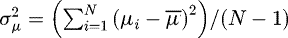 ,
,  is a random error of item j from group i, and
  is a short-term systematic error in group i. Note that the variance of Iij is given by
  . The term
  is the called “product variability” by Grubbs [6]. Neither RIij nor SIi are observable from data. However, for various types of observed data, we can estimate the variances
  and
and  . The same error model is typically also used for the operator, but with
  and
and  . We use capital letters such as I and O to denote random variables and corresponding lower case letters i and o to denote the corresponding observed values.
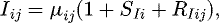
Figure 1 plots simulated example verification measurement data. The relative difference d˜ = (o − i)/o is plotted for each of 10 paired (o,i) measurements in each of 5 groups (inspection periods), for a total of 50 relative differences. As shown in Figure 1, typically, the between-group variation is noticeable compared to the within-group variation, although the between-group variation is amplified to a quite large value for better illustration in Figure 1; we used δRO = 0.005, δSO = 0.001, δRI = 0.01, δSI = 0.03, and the value δSI = 0.03 is quite large. Figure 2a is the same type of plot as Figure 1, but is for real data (four operator and inspector measurements on drums of UO2 powder from each of three inspection periods). Figure 2b plots inspector versus operator data for each of the three inspection periods; a linear fit is also plotted.
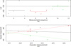 |
Fig. 2 Example real verification measurement data. (a) Four paired (O,I) measurements in three inspection periods; (b) inspector vs. operator measurement by group, with linear fits in each group. |
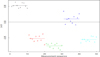 |
Fig. 1 Example simulated verification measurement data. The relative difference d˜ = (o − i)/o is plotted for each of 10 paired (o,i) measurements in each of 5 groups, for a total of 50 relative differences. The mean relative difference within each group (inspection period) is indicated by a horizontal line through the respective group means of the paired differences. |
2.1 Grubbs' estimator for paired (operator, inspector) data
Grubbs introduced a variance estimator for paired data under the assumption that the measurement error model was additive. We have developed new versions of the Grubbs' estimator to accommodate multiplicative error models and/or prior information regarding the relative sizes of the true variances [4,5]. Grubbs' estimator was developed for the situation in which more than one measurement method is applied to multiple test items, but there is no replication of measurements by any of the methods. This is the typical situation in paired (O,I) data.
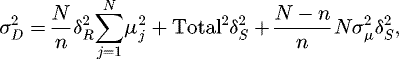
Grubbs' estimator for an additive error model can be extended to apply to the multiplicative model equation (1) as follows. First, equation (1) for the inspector data (the operator data is analysed in the same way) implies that the within-group mean squared error (MSE),  , has expectation
 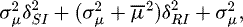 where
where  is the average value of μij (assuming that each group has the same number of paired observations n). Second, the between-group MSE,
  , has expectation
  Therefore, both
  and
and  are involved in both the within- and between-groups MSEs, which implies that one must solve a system of two equations and two unknowns to estimate
  and
and  [4,5]. By contrast, if the error model is additive, only
  is involved in the within-group MSE, while both
  and
and  are involved in the between-group MSE. The term
  in both equations is estimated as in the additive error model, by using the fact that the covariance between operator and inspector measurements equals
  [4,5]. However,
  will be estimated with non-negligible estimation error in many cases. For example, see Figure 2b where the fitted lines in periods 1 and 3 have negative slope, which implies that the estimate of
  is negative in periods 1 and 3 (but the true value of
  cannot be negative in this situation). We note that in the limit as
  approaches zero, the expression for the within-group MSE reduces to that in the additive model case (and similarly for the between-group MSE).
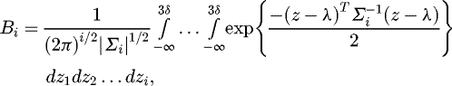
3 Applying uncertainty estimates: the D statistic and one-at-a-time-verification measurements
This paper considers two possible IAEA verification tests. First, the overall D test for a pattern is based on the average difference,  . Second, the one-at-a-time test compares the operator to the corresponding inspector measurement for each item and a relative difference is computed, defined as dj = (oj − ij)/oj. If dj > 3δ, where
  where
where  and
and  (or some other alarm threshold close to the value of 3 that corresponds to a small false alarm probability), then the jth item selected for verification leads to an alarm. Note that the correct normalization used to define the relative difference is actually dj = (oj − ij)/μj, which has standard deviation exactly δ. But μj is not known in practice, so a reasonable approximation is to use dj = (oj − ij)/oj, because the operator measurement oj is typically more accurate and precise than the inspectors's NDA measurement ij. Provided
  (approximately), one can assume that dj = (oj − ij)/oj is an adequate approximation to dj = (oj − ij)/μj [10]. Although IAEA experience suggests that
  sometimes exceeds 0.20, usually
 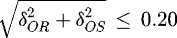 [8].
[8].
3.1 The D statistic to test for a trend in the individual differences dj = oj − ij
For an additive error model, Iij = μij + SIi + RIij, it is known [11] that the variance of the D statistic is given by  , where
 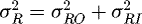 and
and 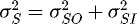 are the absolute (not relative) variances. If one were sampling from a finite population without measurement error to estimate a population mean, then
  where f = (N − n)/N is the finite population correction factor, and σ2 is a quasi-variance term (the “item variance” as defined previously in a slightly different context), defined here as
 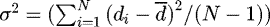 . Notice that without any measurement error, if n = N then f = 0, so
  , which is quite different from
  . Figure 1 can be used to explain why
 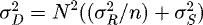 when there are both random and systematic measurement errors. And, the fact that
 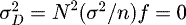 when n = N and there are no measurement errors is also easily explainable.
For a multiplicative error model (our focus), it can be shown [11] that
 (2)
where
(2)
where  and
and  , and so to calculate
  in equation (2), one needs to know or assume values for
  (the item variance) and the average of the true values,
  . In equation (2), the first two terms are analogous to
  in the additive error model case. The third term involves
  and decreases to 0 when n = N. Again, in the limit as
  approaches zero, equation (2) reduces to that for the additive model case; and regardless whether
  is large or near zero, the effect of
  cannot be reduced by taking more measurements (increasing n in Eq. (2)).
In general, the multiplicative error model gives different results than an additive error model because variation in the true values,  , contributes to
  in a multiplicative model, but not in an additive model. For example, let
  and
and  , so that the average variance in the multiplicative model is the same as the variance in the additive model for both random and systematic errors. Assume δR = 0.10, δS = 0.02,
  (arbitrary units), and
  (50% relative standard deviation in the true values). Then the additive model has σD = 270.8 and the corresponding multiplicative model with the same average absolute variance has σD = 310.2, a 15% increase. The fact that var(μ) contributes to
  in a multiplicative model has an implication for sample size calculations such as those we describe in Section 4. Provided the magnitude of SIij + RIij is approximately 0.2 or less (equivalently, the relative standard deviation of SIij + RIij should be approximately 8% or less), one can convert equation (1) to an additive model by taking logarithms, using the approximation log(1 + x) ≈ x for |x| ≤ 0.20. However, there are many situations for which the log transform will not be sufficiently accurate, so this paper describes a recently developed option to accommodate multiplicative models rather than using approximations based on the logarithm transform [4,5].
The overall D test for a pattern is based on the average difference, 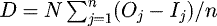 . The D-statistic test is based on equation (2), where
  is the random error variance and
  is the systematic error variance of d˜ = (o − i)/μ ≈ (o − i)/o, and
  is the absolute variance of the true (unknown) values. If the observed D value exceeds 3σD (or some similar multiple of σD to achieve a lot false alarm probability) then the D test alarms.
The test that alarms if D ≥ 3σD is actually testing whether D ≥ 3σˆD, where σˆD denotes an estimate of σD; this leads to two sample size evaluations. The first sample size n1 involves metrology data collected in previous inspection samples used to estimate 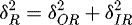 ,
,  , and
, and  needed in equation (2). The second sample size n2 is the number of operator's declared measurements randomly selected for verification by the inspector. The sample size n1 consists of two sample sizes: the number of groups g (inspection periods) used to estimate
  and the total number of items over all groups, n1 = gn in the case (the only case we consider in examples in Sect. 4) that each group has n paired measurements.
3.2 One-at-a-time sample verification tests
The IAEA has historically used zero-defect sampling, which means that the only acceptable (passing) sample is one for which no defects are found. Therefore, the non-detection probability is the probability that no defects are found in a sample of size n when one or more true defective items are in the population of size N. For one-item-at-a-time testing, the non-detection probability is given by
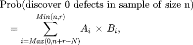 (3)
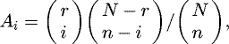
where the term Ai is the probability that the selected sample contains i truly defective items, which is given by the hypergeometric distribution with parameters on i, n, N, r, where i is the number of defects in the sample, n is the sample size, N is the population size, and r is the number of defective items in the population. More specifically,
(3)
where the term Ai is the probability that the selected sample contains i truly defective items, which is given by the hypergeometric distribution with parameters on i, n, N, r, where i is the number of defects in the sample, n is the sample size, N is the population size, and r is the number of defective items in the population. More specifically,
 the above equation is the probability of choosing i defective items from r defective items in a population of size N in a sample of size n, which is the well-known hypergeometric distribution. The term Bi is the probability that none of the i truly defective items is inferred to be defective based on the individual d tests. The value of Bi depends on the metrology and the alarm threshold. Assuming a multiplicative error model for the inspector measurement (and similarly for the operator), implies that, for an alarm threshold of k = 3, for
  we have to calculate
  , where
 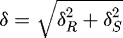 , which is given by the multivariate normal integral
 where each of the components of λ are equal to 1 SQ/r (SQ is a significant quantity; for example, 1 SQ = 8 kg for Pu, and r was defined above as the number of defective items in the population). The term ∑i in the Bi calculation involved in the multivariate normal integral is a square matrix with i rows and columns with values
  on the diagonal and values
  on the off-diagonals.
4 Simulation study
The left hand side of equations (2) and (3) can be considered a “measurand” in the language used in the guide to expressing uncertainty in measurement [12]. Although the error propagation in the GUM is typically applied in a “bottom-up” uncertainty evaluation of a measurement method, it can also be applied to any other output quantity y (such as y = σD or y = DP) expressed as a known function y = f(x1, x2, …, xp) of inputs x1, x2, …, xp (inputs such as 
 and
and  ). The GUM recommends linear approximations (“delta method”) or Monte Carlo simulations to propagate uncertainties in the inputs to predict uncertainties in the output. Here we use Monte Carlo simulations to evaluate the uncertainties in the inputs
 and
and  and also to evaluate the uncertainty in y = σD or y = DP as a function of the uncertainties in the inputs. Notice that equation (2) is linear in
  and
and  so the delta method to approximate the uncertainty in y = σD would be exact; however, there is non-zero covariance (a negative covariance) between
  and
and  that would need to be taken into account in the delta method.
We used the statistical programming language R [13] to perform simulations for example true values of  , and the amount of diverted nuclear material. For each of 105 or more simulation runs, normal errors were generated assuming the multiplicative error model (1) for both random and systematic errors (see Sect. 4.2 for examples with non-normal errors). The new version of the Grubbs' estimator for multiplicative errors was applied to produce the estimates
  ,
,  ,
,  ,
,  , and
, and  , which were then used to estimate y = σD in equation (2) and y = DP in equation (3). Because there is large uncertainty in the estimates
  ,
,  ,
,  ,
,  unless
  is nearly 0, we also present results for a modified Grubbs' estimator applied to the relative differences
 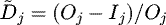 that estimates the aggregated variances
  and
and 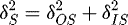 , and also estimates
  . Results are described in Sections 4.1 and 4.2.
4.1 The D statistic to test for a trend in the individual differences dj = (oj − ij)/oj
Figure 3 plots 95% CIs for σD versus sample size n2 using the modified Grubbs' estimator applied to the relative differences  for the parameter values δRO = 0.01, δSO = 0.001, δRI = 0.05, δSI = 0.005,
  , σμ = 0.01, N = 200 for case A (defined here and throughout as n1 = 4 with g = 2, n = 2) and for case B (defined here and throughout as n1 = 50 with g = 5, n = 10) . We used 105 simulations of the measurement process to estimate the quantiles of the distribution of y = σD. We confirmed by repeating the sets of 105 simulations that simulation error due to using a finite number of simulations is negligible. Clearly, and not surprisingly, the sample size in Case A leads to CI length that seems to be too wide for effectively quantifying the uncertainty in σD. The traditional Grubbs' estimator performs poorly unless σμ is very small, such as σμ = 0.0001. We use the traditional Grubbs' estimator in Section 4.2. The modified estimator that estimates the aggregated variances performs well for any value of σμ.
Figure 4 is similar to Figure 3, except Figure 4 plots the length of 95% CIs for 6 possible values of n1 (see the figure legend). Again, the case A sample size is probably too small for effective estimation of σD. In this example, the smallest length CI is for g = 5 and n = 100, but n = 100 is unrealistically large, while g = 3 and n = 10 or g = 5 and n = 10 are typically possible with reasonable resources. The length of these 95% CIs is one criterion to choose an effective sample size n1.
Another criterion to choose an effective sample size n1 is the root mean squared error (RMSE, defined below) in estimating the sample size n2 needed to achieve σD = 8/3.3 (the 3.3 is an example value that corresponds to a 95% DP to detect an 8 kg shift (1 SQ for Pu) while maintaining a 0.05 FAP when testing for material loss). In this example, the RMSE in estimating the sample size n2 needed to achieve σD = 8/3.3 is approximately 12.9 for case A and 8.0, 7.3, 6.8, 6.7, and 6.3, respectively, for the other values of n1 considered in Figure 4. These RMSEs are repeatable to within ±0.1 across sets of 105 simulations so the RMSE values are in the same order as the CI lengths in Figure 4. The RMSE is defined as
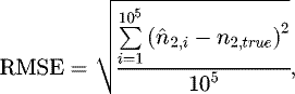 where nˆ2,i is the estimated sample size n2 in simulation i that is needed in order to achieve σD = 8/3.3, and n2,true is the true sample size n2 (n2,true = 22 in this example; see Fig. 3 where the true value of σD versus n2 is also shown) needed to achieve σD = 8/3.3.
Another criterion to choose an effective size n1 is the detection probability to detect specified loss scenarios. We consider this criterion in Section 4.3.
 |
Fig. 3 The estimate of σD versus sample size n2 for two values of n1 (case A: g = 2, n = 2 so n1 = 4, or case B: g = 5, n = 10 so n1 = 50). |
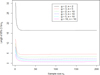 |
Fig. 4 Estimated lengths of 95% confidence intervals for σD versus sample size n2 for six values of n1 (g = 2, n = 2 so n1 = 4, g = 3, n = 5 so n1 = 15, etc.). |
4.2 Uncertainty on the uncertainty on the uncertainty
The term “uncertainty” typically refers to a measurement error standard deviation, such as σD. Therefore, Figures 3 and 4 involve the “uncertainty of the uncertainty” as a function of n1 (defined as n1 = ng, so more correctly, as a function of g and n) and n2. Figures 5–7 illustrate the “uncertainty of the uncertainty of the uncertainty” (we commit to stopping at this level-three usage of “uncertainty”). The “uncertainty of the uncertainty” depends on the underlying measurement error probability density, which is sometimes itself uncertain. Figure 5 plots the familiar normal density and three non-normal densities (uniform, gamma, and generalized lambda, [14]). Figure 6 plots the estimated probability density (using the 105 realizations) of the estimated value of δIR using the traditional Grubbs' estimator for each of the four distributions (the true value of δIR is 0.05) and the five true standard deviations are the same as in Section 4.1 for generating the random variables (δRO = 0.01, δSO = 0.001, δRI = 0.05, δSI = 0.005,  , σμ = 0.01, N = 200). Figure 7 is similar to Figure 3 (for g = 5, n = 10), except it compares CIs assuming the normal distribution to CIs assuming the generalized lambda distribution. That is, Figure 7 plots the estimated CI, again for the model parameters as above, for σD for the normal and for the generalized lambda distributions. In this case, the CIs are wider for the generalized lambda distribution than for the normal distribution. Recall (Fig. 5) that standard deviation of the four estimated probability densities are: 0.14, 0.25, 0.10, and 0.36 for the normal, gamma, uniform, and generalized lambda, respectively. Therefore, one might expect the CI for σD to be shorter for the normal than for a generalized lambda distribution that has the same relative standard deviation as the corresponding normal distribution.
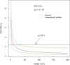 |
Fig. 7 95% confidence intervals for the estimate of σD versus sample size n2 for case B, assuming the measurement error distribution is either the normal or the generalized lambda distribution. |
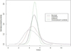 |
Fig. 6 The estimated probability density for δˆIR in the four example measurement error probability densities (normal, gamma, uniform, and generalized lambda, each with mean 0 and variance 1) from Figure 4. |
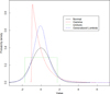 |
Fig. 5 Four example measurement error probability densities: normal, gamma, uniform, and generalized lambda, each with mean 0 and variance 1. |
4.3 One-at-a-time testing
For one-at-a-time testing, Figure 8 plots 95% confidence intervals for the estimated DP versus sample size n2 for cases A and B (see Sect. 4.1). The true parameter values used in equation (3) were δRO = 0.1, δSO = 0.05, δRI = 0.1, δSI = 0.05,  , σμ = 0.01. And, a true mean shift of 8 kg in each of 10 falsified items was used (representing data falsification by the operator to mask diversion of material). The CIs for the DP were estimated by using the observed 2.5% and 97.5% quantiles of the DP values in 105 simulations. As in Section 4.1, we confirmed by repeating the sets of 105 simulations that simulation error due to using a finite number of simulations is negligible. The very small case A sample leads to approximately the same lower 2.5% quantile as did case B; however, the upper 97.5% quantile is considerably lower for case A than for case B. Other values for the parameters (δRO, δSO, δRI, δSI,
  , σμ, the number of falsified items, and the amount falsified per item) lead to different conclusions about uncertainty as a function of n2 in how the DP decreases as a function of n2. For example, if we reduce
  to
to  in this example, then the confidence interval lengths are very short for both case A and case B.
For this same example, we can also compute the DP in using the D statistic to detect the loss (which the operator attempts to mask by falsifying the data). For the example just described (for which simulation results are shown in Fig. 8), the true DP in using the D statistic (using an alarm threshold of σD and n2 = 30 using Eq. (2)) is 0.65. The corresponding true DP for one-at-a-time testing is 0.27. Therefore, in this example, with 10 of 200 items falsified, each by an amount of 8 units, the D statistic has lower DP than the n2 = 30 one-at-a-time tests. In other examples, the D statistic will have higher DP, particularly when there are many falsified items in the population. For example, if we increase the number of defectives in this example from 10 of 200 to 20, 30, or 40 of 200, then the DPs are (0.17, 0.17), (0.08, 0.15), and (0.06, 0.14) for one-at-a-time testing and for the D statistic, respectively. These are low DPs, largely because the measurement error variances are large in this example. One can also assess the sensitivity of the estimated DP in using the D statistic to the uncertainty in the estimated variances; for brevity, we do not show that here.
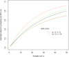 |
Fig. 8 Estimated detection probability and 95% confidence interval versus sample size n2 for cases A and B. The true detection probability is plotted as the solid (black) line. |
5 Discussion and summary
This study was motivated by three considerations. First, there is an ongoing need to improve UQ for error variance estimation. For example, some applications involve characterizing items for long-term storage and the measurement error behaviour for the items is not well known, so an initial metrology study with to-be-determined sample sizes is required. Second, we recently provided the capability to allow for multiplicative error models in evaluating the D statistic (Eq. (2)) [4,5]. Third, we recently provided the capability to allow for both random and systematic errors in one-at-a-time item testing (Eq. (3)).
We presented a simulation study that assumed error variances are estimated using an initial metrology study characterized by g measurement groups and n paired operator, inspector measurements per group. Not surprisingly, both one-item-at-a-time testing and pattern testing using the D statistic, it appears that g = 2 and n = 2 is too small for effective variance estimation.
Therefore, the sample sizes in the previous and current inspections will impact the estimated DP and FAP, as is illustrated by numerical examples. The numerical examples include application of the new expression for the variance of the D statistic assuming the measurement error model is multiplicative (Eq. (2)) is used in a simulation study and new application of both random and systematic error variances in one-item-at-a-time testing (Eq. (3)).
Future work will evaluate the impact of larger values of product variability,  on the standard Grubbs' estimator; this study used a very small value of
  , which is adequate in some contexts, such as product streams. The value of
  could be considerably larger in some NM streams, particularly waste streams. Therefore, this study also evaluated the relative differences dj = (oj − ij)/oj to estimate the aggregated quantities needed in equations (2) and (3),
  , using a modified Grubbs' estimation, to mitigate the impact of noise in estimation of σμ. Because
  is a source of noise in estimating the individual measurement error variances [15], a Bayesian alternative is under investigation to reduce its impact [16]. Also, one could base a statistical test for data falsification based on the relative differences between operator and inspector measurements d = (o − i)/o in which case an alternate expression to equation (2) for σD that does not involve the product variability
  would be used.
5.1 Implications and influences
This study was motivated by three considerations, each of which have implications for future work. First, there is an ongoing need to improve UQ for error variance estimation. For example, some applications involve characterizing items for long-term storage and the measurement error behaviour might not be well known for the items, so an initial metrology study with to-be-determined sample sizes is required. Second, we recently provided the capability to allow for multiplicative error models in evaluating the D statistic (Eq. (2) in Sect. 3) [4,5]. Third, we recently provided the capability to allow for both random and systematic errors in one-at-a-time item testing (Eq. (3) in Sect. 3). Previous to this work, the variance of the D statistic was estimated by assuming measurement error models are additive rather than multiplicative, and one-at-a-time item testing assumed that all measurement errors were purely random.
Acknowledgments
The authors acknowledge CETAMA for hosting the November 17–19, 2015 conference on sampling and characterizing where this paper was first presented.
References
- R. Avenhaus, M. Canty, Compliance Quantified (Cambridge University Press, 1996) [CrossRef] [Google Scholar]
- T. Burr, M.S. Hamada, Revisiting statistical aspects of nuclear material accounting, Sci. Technol. Nucl. Install. 2013, 961360 (2013) [Google Scholar]
- T. Burr, M.S. Hamada, Bayesian updating of material balances covariance matrices using training data, Int. J. Prognost. Health Monitor. 5, 6 (2014) [Google Scholar]
- E. Bonner, T. Burr, T. Guzzardo, T. Krieger, C. Norman, K. Zhao, D.H. Beddingfield, W. Geist, M. Laughter, T. Lee, Ensuring the effectiveness of safeguards through comprehensive uncertainty quantification, J. Nucl. Mater. Manage. 44, 53 (2016) [Google Scholar]
- T. Burr, T. Krieger, K. Zhao, Grubbs' estimators in multiplicative error models, IAEA report, 2015 [Google Scholar]
- F. Grubbs, On estimating precision of measuring instruments and product variability, J. Am. Stat. Assoc. 43, 243 (1948) [CrossRef] [Google Scholar]
- K. Martin, A. Böckenhoff, Analysis of short-term systematic measurement error variance for the difference of paired data without repetition of measurement, Adv. Stat. Anal. 91, 291 (2007) [CrossRef] [Google Scholar]
- R. Miller, Beyond ANOVA: Basics of Applied Statistics (Chapman & Hall, 1998) [Google Scholar]
- C. Norman, Measurement errors and their propagation, Internal IAEA Document, 2014 [Google Scholar]
- G. Marsaglia, Ratios of normal variables, J. Stat. Softw. 16, 2 (2006) [Google Scholar]
- T. Burr, T. Krieger, K. Zhao, Variations of the D statistics for additive and multiplicative error models, IAEA report, 2015 [Google Scholar]
- Guide to the Expression of Uncertainty in Measurement, JCGM 100: www.bipm.org (2008) [Google Scholar]
- R Core Team R, A Language and Environment for Statistical Computing (R Foundation for Statistical Computing, Vienna, Austria, 2012): www.R-project.org [Google Scholar]
- M. Freimer, G. Mudholkar, G. Kollia, C. Lin, A study of the generalized Tukey Lambda family, Commun. Stat. Theor. Methods 17, 3547 (1988) [CrossRef] [Google Scholar]
- F. Lombard, C. Potgieter, Another look at Grubbs' estimators, Chemom. Intell. Lab. Syst. 110, 74 (2012) [CrossRef] [Google Scholar]
- C. Elster, Bayesian uncertainty analysis compared to the application of the gum and its supplements, Metrologia 51, S159 (2014) [CrossRef] [Google Scholar]
Cite this article as: Tom Burr, Thomas Krieger, Claude Norman, Ke Zhao, The impact of metrology study sample size on uncertainty in IAEA safeguards calculations, EPJ Nuclear Sci. Technol. 2, 36 (2016)
All Figures
|
Fig. 2 Example real verification measurement data. (a) Four paired (O,I) measurements in three inspection periods; (b) inspector vs. operator measurement by group, with linear fits in each group. |
| In the text | |
|
Fig. 1 Example simulated verification measurement data. The relative difference d˜ = (o − i)/o is plotted for each of 10 paired (o,i) measurements in each of 5 groups, for a total of 50 relative differences. The mean relative difference within each group (inspection period) is indicated by a horizontal line through the respective group means of the paired differences. |
| In the text | |
|
Fig. 3 The estimate of σD versus sample size n2 for two values of n1 (case A: g = 2, n = 2 so n1 = 4, or case B: g = 5, n = 10 so n1 = 50). |
| In the text | |
|
Fig. 4 Estimated lengths of 95% confidence intervals for σD versus sample size n2 for six values of n1 (g = 2, n = 2 so n1 = 4, g = 3, n = 5 so n1 = 15, etc.). |
| In the text | |
|
Fig. 7 95% confidence intervals for the estimate of σD versus sample size n2 for case B, assuming the measurement error distribution is either the normal or the generalized lambda distribution. |
| In the text | |
|
Fig. 6 The estimated probability density for δˆIR in the four example measurement error probability densities (normal, gamma, uniform, and generalized lambda, each with mean 0 and variance 1) from Figure 4. |
| In the text | |
|
Fig. 5 Four example measurement error probability densities: normal, gamma, uniform, and generalized lambda, each with mean 0 and variance 1. |
| In the text | |
|
Fig. 8 Estimated detection probability and 95% confidence interval versus sample size n2 for cases A and B. The true detection probability is plotted as the solid (black) line. |
| In the text | |
Current usage metrics show cumulative count of Article Views (full-text article views including HTML views, PDF and ePub downloads, according to the available data) and Abstracts Views on Vision4Press platform.
Data correspond to usage on the plateform after 2015. The current usage metrics is available 48-96 hours after online publication and is updated daily on week days.
Initial download of the metrics may take a while.