© E. K. Njayou Tsepeng et al., Published by EDP Sciences, 2025

1. Introduction

In reactor physics field, the qualification of a calculation code used in operating safety demonstration is pronounced by the operator on the basis of the elements obtained through a three-stage process: Verification, Validation, and Uncertainty Quantification, known as VVUQ, for a specific field of application. The verification stage consists in checking the algorithmic implementation while the validation process, which is more physical, consists in ensuring that the code reproduces the physical phenomena simulated and relies either on comparisons between calculations and measurements (experimental validation) or on comparaisons to reference codes such as Monte Carlo codes (numerical validation). Finally, the uncertainty quantification stage quantifies the various sources of uncertainty and demonstrates that reactor operation under the specified conditions will meet the safety requirements with a certain degree of confidence. In its reference “Guide 28” document [1] related to the qualification of calculation codes used in the safety demonstration, the French Safety Authority discusses about the transposition as a way of extending the domain of use of a calculation code from its initial domain of validation. Even though transposition can be realized by different ways, the most commonly used methods rely on bayesian inference [2]. It consists in transfering information assimilated from one or several well instrumented configurations to a non instrumented one. It is used to infer the behavior of a configuration under unknown conditions, or the relevance of a target design relative to known ones but can also be used for bias and uncertainty reductions.

The use of transposition in neutronics goes back a long way, as can be seen, for example, in Gandini's work in the 1980s [2, 3]. Mainly used in the field of experimental research, it has yielded satisfactory results, especially for designing new critical mock-up experimental programs [4, 5]. Initially applied in Fast Reactors applications [6, 7], this method has later been extended to LWRs and holds significant promises for industrial applications [8, 9], especially for new reactor concepts or non instrumented operating domains of existing reactors (e.g., accidental situations). Therefore, increasingly stringent safety requirements are prompting operators to explore such methods. The added value will then be to take advantage of the measurements from reactors in operation beside those obtained in critical mock-ups, in order to improve the predictability of industrial simulation tools, which are known for some operational simplifications in formalisms. However, our paper will be essentially focused on the determination of representativity coefficients (degree of similarity) between some mock-up experiments and potential industrial LWR applications, letting the transposition stage for future work.

Our study extends the validation domain of two GenIII target cores, part of the UAM benchmark [10], by including a burnup analysis, not foreseen initially. This study will also enable to determine what is the range of representativity of a zero power reactor (ZPR) without burnup indicator versus cycle burnup. Moreover, ZPR experiments were designed for the purpose of keff, reactivity effects and local pin-by-pin power distributions, it is the first time they are used outside their initial domain, ie the extension to large cores. The present study is thus a first attempt to test the limits of ZPR use in transposition studies.

In this paper, we first present a brief review of the mathematical background, based on bayesian inference. Then, the question of covariance matrices of few energetic groups is adressed: two collapsing methodologies, relying on either reaction rates or uncertainty conservation principles are compared and serve to collapse covariance data from a fine to a coarse energy mesh for the sake of the study. The nuclear data sensitivities are derived from the SPT first order [11, 12] for the effective multiplication factor and from the GPT first order [13, 14] for fission rate ratio. Then, the uncertainties are propagated using the Sandwich rule (also known as the delta method in statistics) following some hypothesis and pre-tratments on total scattering covariance data due to code limitations. The effect of the nuclear data perturbation on the isotopic concentrations were not taken into account. Finally, the representativities of several assemblies and full core configurations were performed and analysed. The aim here is to study the relevance and the feasibility of such an approach with an industrial core calculation tool.

All the calculations are performed with the deterministic core code COCAGNE [15], developed jointly by EDF (Electricité De France) and FRAMATOME. A simplified spherical harmonics of order 3 (SP3) [16] solver is used with an 8-group energy mesh. At this stage, integral information has not been integrated into the study and remains the subject of further works.

2. Mathematical background

The knowledge on nuclear data is generally improved thanks to differential and integral experiments. The initial values are updated via data assimilation. The transposition, for its part, takes advantage of this assimilation to improve the knowledge on integral data between different configurations. Both notions are commonly derived from the Bayes’ theorem and are described in the following paragraphs.

There are two types of data assimilation methods [17]. The deterministic approaches are based on the use of approximations and hypotheses allowing for the analytical or numerical solving of equations. They use for example Bayesian inference, maximum likelihood, Lagrange multipliers, or least-square methods (generalized or ordinary). The stochastic approach are based on Monte Carlo sampling of prior distributions. Both approaches are well-known and already used in neutron physics for assimilating nuclear data provided by international libraries. Through iterative adjustments, the aim is to enhance the accuracy of nuclear data from differential or integral experiments. For example, reference [18] compares different methods, both stochastic and deterministic, on a unique test case and highlights the advantages and limitations of each of them.

In this article, we will employ the deterministic method due to a linearity hypothesis between the interest variables y and the nuclear data x. Subsequently, we will utilize Bayesian inference to introduce the equations applied for transposition, focusing particularly on the notion of representativity. It is noteworthy that under the usual hypothesis of Gaussian error in observations, there exists a mathematical equivalence [19, 20] among formulations derived from various methods (GLLS, Least-squares, Maximum Likelihood, Bayesian inference), which are nevertheless referred to by different names in the literature.

2.1. The Bayes’ theorem

Let Y be a continous random variable describing the state of a system, i.e. the interest data. We assume that each realisation of Y depends on X, a vector of continuous random variables representing parameters. Bayes’ theorem is expressed as follows.

If f_X(x) is the prior probability density function of X and if f_Y|X(y|x) is the conditional probability density function of Y given X=x, then, the posterior probability density function of X given Y=y, denoted as f_X|Y(x|y), is given by:

$$f_{\text{X}|Y}(\text{x}|y)=\frac{f_{Y|\text{X}}(y|\text{x})f_{\text{X}}(\text{x})}{f_Y(y)}$$

where f_Y(y) is the marginal probability density function of Y, defined by integrating the joint probability density function f_Y|X(y|x) over all possible values of X, that is:

$$f_Y(y)={\displaystyle {\int }_{\text{x}}}{f}_{Y|\text{X}}(y|\text{x})d\text{x}$$

This theorem describes how the posterior probability density function of X, after observing Y=y, is calculated by integrating the prior probability density function of X, the conditional probability density function (also called the likehood function) of Y given X=x, and normalizing by the marginal probability density function of Y.

2.2. Data assimilation by Bayesian inference: hypothesis of linear model and gaussian distributions

In this article, the quantities of interest Y are the effective multiplication factor and the fission rate ratio, calculated by a neutron deterministic calculation scheme. The input data X are the nuclear data. The measured experimental and calculated values associated with the true unknown value Y are respectively denoted by Y_E and Y_C, such as Y_E=Y+ɛ_E and Y_C=Y+ɛ_C, where ɛ_E and ɛ_C represent the measurement and calculation errors.

The prior distribution represents our initial knowledge of the parameters X before considering the experimental observations. Let's assume a normal prior distribution¹ for X, $\text{X}\sim \mathcal{N}({\text{x}}_0,B_{{\text{X}}_0})$ with x₀ the prior mean of the parameters and $B_{{\text{x}}_0}$ is the prior covariance matrix of the parameters, representing the initial uncertainties.

The likehood model describes how the observations y_E of Y_E are related to the parameters X. To build this model, we use knowledge from the calculation. The sensitivities S of Y_C regarding the nuclear data X are determined with the first order perturbation theory.

Letting y_C=f(x) be the deterministic function associated with the random variable Y_C, such that y₀=f(x₀), we assume that Y_C can be approximated by a first-order Taylor expansion around the nominal values y₀ and x₀:

$$Y_C=y_0+\text{S}(\text{X}-{\text{x}}_0)+{\varepsilon }_{\mathit{Taylor}},$$(1)

where $\text{S}={\left({\left[\frac{\partial f}{\partial x_i}\right]}_{x_i=x_{i0}}\right)}_{i=1\dots d}\in {ℝ}^d$ is the gradient or sensitivity vector of y_C with respect to the d parameters X evaluated at x₀ and ɛ_Taylor represents the error due to the Taylor approximation, which is typically small for small perturbations and can often be neglected under the hypothesis of linearity.

The experimental random variable can then be expressed as:

$$Y_E=y_0+\text{S}(\text{X}-{\text{x}}_0)+\varepsilon ,$$(2)

with ɛ=ɛ_M+ɛ_E and ɛ_M is the modeling bias due to the Taylor approximation and the calculation biases. ɛ_E is assumed a Gaussian and centered random error, i.e., ${\varepsilon }_E\sim \mathcal{N}(0,{\sigma }_{{\varepsilon }_E}^2)$. The conditional model of Y_E given X=x is given such as:

$$Y_E|\text{X}=\text{x}\sim \mathcal{N}(y_0+\text{S}(\text{x}-{\text{x}}_0),{\sigma }_{\varepsilon }^2).$$

The total variance of the C/E ratio results from the sum of ${\sigma }_C^2$ the propagated uncertainty of the parameters X through the model and ${\sigma }_{\varepsilon }^2$ the combined measurement and modeling uncertainties:

$${\sigma }_{C/E}^2={\sigma }_C^2+{\sigma }_{\varepsilon }^2,$$

with ${\sigma }_C^2$ given by sandwich rule:

$${\sigma }_C^2=\text{S}{\text{B}}_{{\text{x}}_0}{\text{S}}^t$$(3)

Finally, applying Bayes’theorem with the conjugate relationship between the normal prior and the normal likelihood allows deriving the posterior distribution analytically. The posterior distribution of X given the experimental observations Y_E=y_E is a normal distribution: $\text{X}|Y_E={\mathit{y}}_E\sim \mathcal{N}({\text{x}}_p,{\text{B}}_{{\text{x}}_p})$, with the following parameters:

• the posterior mean,

  $${\text{x}}_p={\text{x}}_0+{\text{B}}_{{\text{x}}_0}{\text{S}}^t{\left(\text{S}{\text{B}}_{{\text{x}}_0}{\text{S}}^t+{\sigma }_{\varepsilon }^2\right)}^{-1}(y_E-y_0),$$(4)

• and the posterior covariance,

  $${\text{B}}_{{\text{x}}_p}={\text{B}}_{{\text{x}}_0}-{\text{B}}_{{\text{x}}_0}{\text{S}}^t{\left(\text{S}{\text{B}}_{{\text{x}}_0}{\text{S}}^t+{\sigma }_{\varepsilon }^2\right)}^{-1}\text{S}{\text{B}}_{{\text{x}}_0}$$(5)

2.3. Transposition to a case without measure

Let's consider two configurations (a) and (b) for which we want to determine the value of a quantity of interest y and its uncertainty. We know that it is possible to calculate y in both configurations, but only measurements from (a) are known. The transposition method involves using the known measurements from (a) to improve our understanding of (b) and its associated uncertainty. The application of the data assimilation presented in the previous section allows determining the posterior mean and covariance x_p and ${\text{B}}_{{\text{x}}_p}$.

The application of the Taylor approximation (Eq. 1) on the calculation (b) and of the Equation (4) from the data assimilation (a) provide an estimation of the posterior ${\mathit{y}}_p^{(b)}$:

$${\mathit{y}}_p^{(b)}\simeq$$(6)

$${\mathit{y}}_0^{(b)}+{\text{S}}^{(b)}\left[{\text{B}}_{{\text{x}}_0}{{\text{S}}^{(a)}}^t({\text{S}}^{(a)}{\text{B}}_{{\text{x}}_0}{{\text{S}}^{(a)}}^t+{{\sigma }_{\varepsilon }^{(a)}}^2{)}^{-1}({\mathit{y}}_E^{(a)}-{\mathit{y}}_0^{(a)})\right]$$

In the same way, the application of the sandwich rule on the calculation (b) ${\sigma }_{{\mathit{y}}_p}^{(b)}={\text{S}}^{(b)}{\text{B}}_{{\text{x}}_p}{{\text{S}}^{(b)}}^t$ and of the Equation (5) on (a) gives an estimation of the posterior standard deviation due to the propagation of the uncertainties of x_p:

$${\sigma }_{{\mathit{y}}_p}^{(b)}\simeq$$(7)

$${\text{S}}^{(b)}\left[{\text{B}}_{{\text{x}}_0}-{\text{B}}_{{\text{x}}_0}{{\text{S}}^{(a)}}^t({\text{S}}^{(a)}{\text{B}}_{{\text{x}}_0}{{\text{S}}^{(a)}}^t+{{\sigma }_{\varepsilon }^{(a)}}^2{)}^{-1}{\text{S}}^{(a)}{\text{B}}_{{\text{x}}_0}\right]{{\text{S}}^{(b)}}^t$$

Note that we usually do not consider modeling errors in the data assimilation step, i.e ɛ=ɛ_E in Equation (2). By excluding the modeling bias ɛ_M during the Bayesian updating process in Case (a), we ensure that when transposing the improved parameter estimates to Case (b), we avoid propagating biases that are specific to the first case. Each case can independently assess its own modeling bias, ensuring more accurate and context-specific bias corrections.

The representativity between the two cases (a) and (b) is then given by the Pearson correlation, which are expressed using the Taylor approximations of y^(b) and y^(a) (under the linearity hypothesis). It was introduced by [22] and expresses the degree of shared information between the two cases. Its value ranges between −1 and +1:

$$r_{12}=\frac{{\text{S}}^{(a)}{\text{B}}_{{\text{x}}_0}{\text{S}}^{(b{)}^t}}{{\sigma }_C^{(a)}{\sigma }_C^{(b)}},$$(8)

where ${\sigma }_C^{(a)}=\sqrt{{\text{S}}^{(a)}{\text{B}}_{{\text{x}}_0}{\text{S}}^{(a{)}^t}}$ and ${\sigma }_C^{(b)}=\sqrt{{\text{S}}^{(b)}{\text{B}}_{{\text{x}}_0}{\text{S}}^{(b{)}^t}}$ are given by the sandwich (rule Eq. 3) applied on (a) and (b).

Using Equation (8), Equation (6) can finally be reformulated as:

$${\mathit{y}}_p^{(b)}-{\mathit{y}}_0^{(b)}=\frac{r_{12}}{1+\frac{{\sigma }_{\varepsilon }^2}{{{\sigma }_C^{(a)}}^2}}\frac{{\sigma }_C^{(b)}}{{\sigma }_C^{(a)}}({\mathit{y}}_E^{(a)}-{\text{S}}^{(a)}{\text{x}}_0)$$(9)

and Equation (7) as follow:

$${\sigma }_{{\mathit{y}}_p}^{(b)}={\sigma }_C^{(b)}*\sqrt{1-\frac{r_{12}^2}{1+\frac{{\sigma }_{\varepsilon }^2}{{{\sigma }_C^{(a)}}^2}}}$$(10)

This constitutes the framework on which the study has been led. A matrix notation can also be derived from Equations (6) and (7) when many experiments and/or outputs are considered (see for e.g., [2, 23]). However, they are not part of this work and therefore will not be presented here.

2.4. Sensitivities

Depending on the integral outputs, different perturbation theories are applied to compute the nuclear data sensitivities. The principle is to estimate an approximate solution of the perturbed state of a system, due to a small change in its parameters. The formalism was initially proposed by Usachev [11] for reactivity and related variables. He then generalized it for ratios of linear functionals of the forward flux [14] and Gandini [13] extended it to any ratio of bilinear functional of the forward and adjoint fluxes.

The first order Standard Perturbation Theory (SPT) was reformulated from Usachev's work by Williams [12] and is used in this work to compute the effective multiplication factor (k) sensitivities to nuclear data (x), expressed in the relative form by Equation (11).

$$\begin{array}{cc}\hfill \tilde{S}(k,x)=\frac{\delta k/k}{\delta x/x}\hspace{0.5em}& =\frac{k·\delta \rho }{p}\hfill \\ \hfill & =\hspace{0.5em}\frac{\langle {\varphi }^{*},(\delta F-k\delta L)\varphi \rangle }{p\hspace{0.5em}·\hspace{0.5em}\langle {\varphi }^{*},F\varphi (x)\rangle }\hfill \end{array}$$(11)

where p represents the relative perturbation (δx/x), ϕ, ϕ^* respectively the forward and adjoint fluxes and δF, δL are respectively the variations of production and loss operators of the Boltzmann equation due to the change in the parameter x.

If we denote $R=\frac{\langle {\sigma }_n,\varphi \rangle }{\langle {\sigma }_d,\varphi \rangle }$ a reaction rate ratio, the relative sensitivities are computed thanks to the first order Generalized Perturbation Theory (GPT) are expressed in Equation (12):

$$\begin{array}{cc}\hfill \tilde{S}(R,x)\hspace{0.5em}& =\frac{\delta R/R}{\delta x/x}\hfill \\ \hfill & =\hspace{0.5em}\frac{1}{p}·\left(\frac{\langle \delta {\sigma }_n,\varphi \rangle }{\langle {\sigma }_n,\varphi \rangle }-\frac{\langle \delta {\sigma }_d,\varphi \rangle }{\langle {\sigma }_d,\varphi \rangle }\right)\hfill \\ \hfill \hspace{0.5em}& \hspace{0.5em}-\frac{1}{p}·\left(\langle \mathrm{\Gamma },(\delta {\text{L}}^{*}-\frac{\delta {\text{F}}^{*}}{k}){\varphi }^{*}\rangle \right)\hfill \end{array}$$(12)

where σ_n and σ_d are respectively the numerator and denominator sections and Γ is a Lagrangian multiplier verifying:

$$\{\begin{array}{cc}(\text{L}-\frac{\text{F}}{k})\mathrm{\Gamma }=\frac{\partial f}{\partial {\mathrm{\Psi }}^{*}}\hfill & \hfill \\ \hfill & \hfill \\ <\mathrm{\Gamma },{\text{F}}^{*}{\mathrm{\Psi }}^{*}>=0\hfill & \hfill \end{array}$$

also called the forward importance function related to R (see [13] for more detail). Γ is often interpreted as the indirect contribution on δR accounting for the change in the forward flux, due to the nuclear data perturbation. The first term of the second member of Equation (12) is called the direct effect while the second is called the indirect effet of the perturbation. Some interesting core parameters are covered by this formalism such as local reaction rate ratios, relative power distribution, axial offset or kinetics parameters.

These equations rely on a first order (linear) perturbation theory and the reliability of the prediction might be questionable when some large changes are applied on the parameters. As a response, Weisbin [24] has compared the sensitivity analysis prediction versus a direct calculation after doubling an influential cross-section of his study from one hand, and after changing the cross-section data files from the other hand. Several performance outputs were considered and it was shown that linear perturbation theory predicts the changes in calculated results very satisfactorily. Generally, it is assumed that uncertainties in the cross-sections of interest for core physics applications are in the range for which linear sensitivity theory is accurate enough [25]. However, a care must be taken for some nuclear data or in the case of advanced reactors, transient behaviour, or even atypical LWR core configurations (see for example [26] in the case of ²³⁸U inelastic cross section), for which the uncertainties can lead to non-linearities, and are therefore ill-suited to first-order perturbation theory. This is why efforts to continuously improve nuclear data are a necessity in reactor physics.

3. Results and analysis

The study has been realized in two phases: firstly, single assemby calculations served to set up the procedure and evaluate the different hypotheses and pre-treatments which were then applied for core level calculations. They are presented and discussed in the following paragraphs.

For each calculation, the multigroup nuclear data libraries were generated using the CARABAS lattice code based on APOLLO2 [27], following a two-level scheme [28] and the milti-group cross-sections were condensed to 8 groups on a cell-by-cell spatial mesh. In concrete terms, from the CEAv520² nuclear data library (a few hundred groups) processed by the NJOY processing code [29] at the French Atomic Energy Commission (CEA), a 2D calculation with detailed description of the geometry (pellet, cladding, moderator) in infinite medium is realized for each assembly. The first step consists in self-shielding calculation with a P_ij solver and the SHEM reference energy mesh [30]. It is followed by 36-group flux calculation with self-shielded cross-sections, using a MOC (Method Of Caracteristics) solver [31]. At the end of this stage, libraries of multigroup effective cross-sections are condensed to 8-group energy mesh for core calculation. Moreover, equivalence factors are calculated using the superhomogenisation technique (SPH) [32] and enable the reaction rates between the heterogeneous transport of the lattice calculation and the homogeneous transport of the core calculation to be conserved when using the new condensed 8-group nuclear data.

3.1. Single assembly computations: setting the hypotheses and computational procedure

The first part of this work was carried out at fuel assembly scale. Four different PWR-type (Pressurized Water Reactor) assemblies were selected, with different fuel types and enrichments. The material and geometric description are presented in Tables 1 and 2 and can also be found in the Gen-III UAM benchmarks, defined within the framework of an international scientific collaboration under the auspices of the OECD/NEA [10]. Figure 1 shows a 2D cross-section of those assemblies.

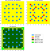Fig. 1. Some UAM GEN-III fuel assemblies.

The UGD_420 assembly contains 12 poisonned rods with 8% of Gd₂O₃ on a 2.2% enriched UO₂. The other rods are 4.2% enriched UO₂ rods. The MOX assembly is a threezoned assembly containing fuel rods with different plutonium contents (9.8%, 6.5% and 3.7%). All calculations were made with a SP3 simplified transport calculation scheme, in an 8 energy groups mesh, at hot zero power (HZP) and critical leakage conditions. The nuclear data library is based on the JEFF3.1.1 evaluation [33].

3.1.1. Covariances for sensitivity and uncertainty analysis

The neutronic errors covariance matrices are from the COMAC database [34] and are generated with the CONRAD code [35] and the ERRORR module of NJOY³. The question of few groups covariance data remains a tricky question. In this paper, we have studied two different ways of collapsing covariance matrices, both based on a different conservation principle.

The first one conserves the reaction rates as indicated in Equation (13):

$${\sigma }_G^r=\frac{{\displaystyle \sum _g}{\sigma }_g^r·{\varphi }_g}{{\displaystyle \sum _g}{\varphi }_g}\hspace{0.5em}\hspace{0.5em}\text{with}\hspace{0.5em}\hspace{0.5em}G=\bigcup _k{g}_k$$(13)

where g is an energy group in the fine energy mesh and G the corresponding group in the coarse one. ${\sigma }_g^r$ is the cross-section of the reaction r in group g. Therefore, the covariance between 2 cross-sections, in the coarse mesh, is expressed by Equation (14)

$$\begin{array}{cc}\hfill \mathit{cov}({\sigma }_G^r,\hspace{0.5em}{\sigma }_{G^{\prime }}^j)=\mathit{cov}\left(\frac{{\displaystyle \sum _g}{\sigma }_g^r·{\varphi }_g}{{\displaystyle \sum _g}{\varphi }_g},\hspace{0.5em}\hspace{0.5em}\frac{{\displaystyle \sum _{g^{\prime }}}{\sigma }_{g^{\prime }}^j·{\varphi }_{g^{\prime }}}{{\displaystyle \sum _{g^{\prime }}}{\varphi }_{g^{\prime }}}\right)& \hfill \end{array}$$(14)

Now assuming the random variable variations are more significant than those of the flux, Equation (14) can be written as:

$$\mathrm{cov}({\sigma }_G^r,\hspace{0.5em}{\sigma }_{G^{\prime }}^j)={\displaystyle \sum _{\genfrac{}{}{0ex}{}{g\in G}{g^{\prime }\in G^{\prime }}}}\frac{{\varphi }_g·{\varphi }_{g^{\prime }}}{{\varphi }_G·{\varphi }_{G^{\prime }}}·\mathrm{cov}\left({\sigma }_g^r,\hspace{0.5em}{\sigma }_{g^{\prime }}^j\right)$$(15)

with ${\varphi }_{G(G^{\prime })}={\displaystyle \sum _{g(g^{\prime })}}{\varphi }_{g(g^{\prime })}$ the flux in the coarse energy mesh.

As in this work we are dealing with relative covariances, i.e. rcov such that: $\mathrm{rcov}\left({\sigma }_g^r,\hspace{0.5em}{\sigma }_{g^{\prime }}^j\right)=\mathrm{cov}\left({\sigma }_g^r,\hspace{0.5em}{\sigma }_{g^{\prime }}^j\right)·{\sigma }_g^r·{\sigma }_{g^{\prime }}^j$ Equation (15) is rewritten as follow:

$$\mathrm{rcov}({\sigma }_G^r,\hspace{0.5em}{\sigma }_{G^{\prime }}^j)={\displaystyle \sum _{\genfrac{}{}{0ex}{}{g\in G}{g^{\prime }\in G^{\prime }}}}\frac{{\tau }_g^r·{\tau }_{g^{\prime }}^j}{{\tau }_G^r·{\tau }_{G^{\prime }}^j}·\mathrm{rcov}\left({\sigma }_g^r,\hspace{0.5em}{\sigma }_{g^{\prime }}^j\right)$$(16)

where τ represents the reaction rate of the corresponding reactions in the corresponding groups. Equation (16) (as Eq. 15) is valid when the covariance involves cross-sections. In the case of normalized fission spectrum (χ), which are real probabilities, the expression is as follow:

$$\mathit{rcov}({\chi }_G,\hspace{0.5em}{\chi }_{G^{\prime }})={\displaystyle \sum _{\genfrac{}{}{0ex}{}{g\in G}{g^{\prime }\in G^{\prime }}}}\frac{{\chi }_g·{\chi }_{g^{\prime }}}{{\chi }_G·{\chi }_{G^{\prime }}}·\mathit{rcov}\left({\chi }_g,\hspace{0.5em}{\chi }_{g^{\prime }}\right)$$(17)

Given an integral parameter, the second is based on a total uncertainty conservation principle, expressed by Equation (18) and derived from Equation (3).

$$\begin{array}{cc}\hfill {\sigma }_C^2& ={\displaystyle {\displaystyle \sum _g}}{S}_g^r·\mathit{cov}\left({\sigma }_g^r,\hspace{0.5em}{\sigma }_{g^{\prime }}^j\right)·S_{g^{\prime }}^j\hfill \\ \hfill & ={\displaystyle {\displaystyle \sum _G}}{S}_G^r·\mathrm{cov}\left({\sigma }_G^r,\hspace{0.5em}{\sigma }_{G^{\prime }}^j\right)·S_{G^{\prime }}^j\hfill \end{array}$$(18)

where $S_g^r$ is the sensitivity of the output Y to reaction r in group g. The decomposition of Equation (18) leads to the expression of $\mathit{cov}\left({\sigma }_G^r,\hspace{0.5em}{\sigma }_{G^{\prime }}^j\right)$ in the coarse energy mesh as follow:

$$\mathrm{cov}({\sigma }_G^r,\hspace{0.5em}{\sigma }_{G^{\prime }}^j)={\displaystyle \sum _{\genfrac{}{}{0ex}{}{g\in G}{g^{\prime }\in G^{\prime }}}}\frac{S_g^r·S_{g^{\prime }}^j}{S_G^r·S_{G^{\prime }}^j}·\mathrm{cov}\left({\sigma }_g^r,\hspace{0.5em}{\sigma }_{g^{\prime }}^j\right)$$(19)

As in the previous cases, when dealing with relative covariances and relative sensitivities (as in this work), Equation (19) becomes:

$$\mathrm{rcov}({\sigma }_G^r,\hspace{0.5em}{\sigma }_{G^{\prime }}^j)={\displaystyle \sum _{\genfrac{}{}{0ex}{}{g\in G}{g^{\prime }\in G^{\prime }}}}\frac{{\tilde{S}}_g^r·{\tilde{S}}_{g^{\prime }}^j}{{\tilde{S}}_G^r·{\tilde{S}}_{G^{\prime }}^j}·\mathrm{rcov}\left({\sigma }_g^r,\hspace{0.5em}{\sigma }_{g^{\prime }}^j\right)·\frac{{\mathit{y}}_{\mathit{coarse}}^2}{{\mathit{y}}_{\mathit{fine}}^2}$$(20)

with y_coarse and y_fine, the respective outputs in the coarse and fine meshes. This approach has already been used by [6].

Both formalisms require an overlap between the coarse and the fine energy meshes. Otherwise, an intermediate mesh must be used.

The covariances are collapsed from 36-group COMAC to 8-group mesh and the results on k_eff uncertainties are given in Tables 3 and 4 for the assemblies at 5000 MWd/t. Different sensitivity profiles (one per assembly) have been considered. The reference indicates the 36-group COMAC results.

The propagated uncertainties of Tables 3 and 4 are quite similar despite the different implications of both formalisms.

• On the first hand, weighting by the flux (or rates) implies that the fluctuation of the flux around its reference value is fairly steady with the fluctuation of the perturbed data, which can be considered in agreement with the small perturbation assumption.

• On the second hand, when we collapse by the sensitivities, the implicit consideration is on the bias induced by the energy mesh, which fluctuation is considered fairly steady with the perturbation. In this case, resonances would then have little influence on the propagation result, and this effect should diminish the finer the mesh. This assumption seems to give satisfactory results with regards of the results in Table 4 and those of reference [37].

The two formalisms appear to be equivalent. However, when the sensitivities are used to collapse covariance data, in some cases, convergence issues can arise, particularly for low sensitivity values, and result in inconsistent uncertainty. The latter is one of the points to be kept in mind while using this approach. Therefore, the use of sufficiently sensitive data is recommended in this case.

It can be seen that the uncertainties obtained depend relatively slightly on the nature of the fuel although some larger discrepancies are noted in the MOX case when other profiles are used. This is an important point when we consider that in the case of more complex geometries (core for example), it is not easy to calculate 36-group sensitivity vectors (or flux) due to memory and/or calculation time issues. In this case, a representative profile, from a simpler geometry, can be used.

A detailed analysis points out the main contributors⁴ (see Tab. 5). As expected, the fissile isotopes are the main isotopic contributors and fission and capture cross-sections are the main reactions in addition to the ${}_{}{}^{235}\mathrm{U}$ multiplicity in the UOX cases.

At this stage, the scattering cross-sections have not yet been integrated in the study⁵ due to their particular treatment, and are the concern of the next section.

3.1.2. Nuclear data for sensitivity and uncertainty analysis

The SP3 8-group energy mesh calculation scheme of COCAGNE was designed to propose a reference to the industrial 2-group diffusion theory, using the same calculation tool. So, it inherited the same choices of nuclear data management, which led to make 2 additional pre-treatments analyzed in this section. Firstly, since only the total scattering section is used by the solvers, the elastic and inelastic scattering cross-sections are not treated appart in the lattice code (CARABAS/APOLLO2), which generates the multigroup nuclear data libraries for the core code, where the covariance matrices are given separately (COMAC files). Secondly, the H₂O molecule is also treated as an unique element in the moderator so that ${}_{}{}^1\mathrm{H}$ and ${}_{}{}^{16}\mathrm{O}$ cannot be treated individually.

The pre-treatments consist on one hand, in constructing total diffusion covariance data from elastic and inelastic ones for each isotopes by taking into consideration the correlations with other reactions. Hence, if we denote ${\sigma }_g^d$, ${\sigma }_g^{\mathit{el}}$ and ${\sigma }_g^{\mathit{in}}$ the total, elastic and inelastic scattering cross-sections in group g such that ${\sigma }_g^d={\sigma }_g^{\mathit{el}}+{\sigma }_g^{\mathit{in}}$, by exploiting the bilinearity principle of the covariance function, we can demonstrate that:

$$\mathit{cov}({\sigma }_g^d,{\sigma }_{g^{\prime }}^r)={\displaystyle \sum _{i=\mathit{el},\mathit{in}}}\mathit{cov}({\sigma }_g^i,{\sigma }_{g^{\prime }}^r)$$(21)

in the case of absolute covariances and:

$$\mathit{rcov}({\sigma }_g^d,{\sigma }_{g^{\prime }}^r)={\displaystyle \sum _{i=\mathit{el},\mathit{in}}}\mathit{rcov}({\sigma }_g^i,{\sigma }_{g^{\prime }}^r)·{\sigma }_g^i·{\sigma }_{g^{\prime }}^r$$(22)

with r any other correlated reaction (including scattering reactions).

The total scattering covariance data are then obtained on the fine energy mesh and must be collapsed into the coarse mesh. To do so, we proceed by the flux weighting formalism which implies to determine elastic and inelastic scattering reaction rates. However, as mentioned earlier, only the total scattering reaction rate can be calculated.

To overcome this issue, we can remark that the total scattering reaction rate is the sum of elastic and inelastic scattering reaction rates. Therefore, the relative contributions of the latter (for a unique isotope) can be given as follow:

$$\{\begin{array}{cc}{f}_g(\mathit{el})\hfill & =\frac{{\mathrm{\Sigma }}_g^{\mathit{el}}}{{\mathrm{\Sigma }}_g^{\mathit{el}}+{\mathrm{\Sigma }}_g^{\mathit{in}}}=\frac{{\sigma }_g^{\mathit{el}}}{{\sigma }_g^{\mathit{el}}+{\sigma }_g^{\mathit{in}}}\hfill \\ f_g(\mathit{in})\hfill & =\frac{{\mathrm{\Sigma }}_g^{\mathit{in}}}{{\mathrm{\Sigma }}_g^{\mathit{el}}+{\mathrm{\Sigma }}_g^{\mathit{in}}}=\frac{{\sigma }_g^{\mathit{in}}}{{\sigma }_g^{\mathit{el}}+{\sigma }_g^{\mathit{in}}}=1-f_g(\mathit{el})\hfill \end{array}$$(23)

with

$${\sigma }_g=\frac{{\int }_{\mathrm{\Delta }g}\varphi (E)·\sigma (E)·\mathit{dE}}{{\int }_{\mathrm{\Delta }g}\varphi (E)·\mathit{dE}}$$

the multigroup microscopic cross-sections. Without any possibility to obtain such quantities, we introduced a flat flux by energy group hypothesis to calculate empirical coefficients from international point-wise nuclear data libraries that have been applied to estimate the elastic and inelastic scattering reaction rates that will serve in the collapsing procedure. The coefficients are given in Equation (24)

$$\{\begin{array}{cc}{\tilde{f}}_g(\mathit{el})=\frac{\overline{{\sigma }_g^{\mathit{el}}(E)}}{\overline{{\sigma }_g^{\mathit{el}}(E)}+\overline{{\sigma }_g^{\mathit{in}}(E)}}\hfill & \hfill \\ {\tilde{f}}_g(\mathit{in})=\frac{\overline{{\sigma }_g^{\mathit{in}}(E)}}{\overline{{\sigma }_g^{\mathit{el}}(E)}+\overline{{\sigma }_g^{\mathit{in}}(E)}}=1-{\tilde{f}}_g(\mathit{el})\hfill & \hfill \end{array}$$(24)

with $\overline{{\sigma }_g(E)}$ the mean value of σ in group g. The relative covariance in the coarse mesh is then given by Equation (25)

$$\begin{array}{cc}\hfill \mathit{rcov}({\sigma }_G^d,{\sigma }_{G^{\prime }}^r)={\displaystyle \sum _{i=\mathit{el},\mathit{in}}}{\displaystyle \sum _{\genfrac{}{}{0ex}{}{g\in G}{g^{\prime }\in G^{\prime }}}}\frac{{\tilde{f}}_g(i)·{\tau }_g^d·{\tau }_{g^{\prime }}^r}{{\tilde{f}}_G(i)·{\tau }_G^d·{\tau }_{G\prime }^r}·\mathit{rcov}\left({\sigma }_g^i,{\sigma }_{g^{\prime }}^r\right)& \hfill \end{array}$$(25)

The JEFF-3.3 nuclear data library [38] served as reference to calculate approximate coefficients⁶, which are given in Table 6 for the main heavy nuclei in the 8-group energy mesh.

On the second hand, as ${}_{}{}^1\mathrm{H}$ and ${}_{}{}^{16}\mathrm{O}$ in the moderator cannot be obtained seperately and regarding the predominance of the ${}_{}{}^1\mathrm{H}$ elastic and capture cross-sections, we decided to consider that all the H₂O total scattering and capture sensitivities are due to ${}_{}{}^1\mathrm{H}$⁷.

Finally, we should have in mind that all these coefficients are empirical and a sensitivity study of the latter might be useful to determine their impact on the final uncertainty.

3.1.3. Sensitivities, uncertainties and representativity analysis

Given the previous hypothesis, we computed the uncertainty of the effective multiplication factor on the different assemblies. To do so, we used the UGD_420 assembly at 5000 MWd/t (to produce Pu isotopes) to collapse the covariance matrices using the reaction rate conservation principle. Table 7 shows the final result. The main contributors remain the same and the scattering cross-sections have a limited impact on the uncertainty of such global parameter. It wouldn’t certainly be the case for local parameters such as power distribution or local reaction rate ratios.

As regards the representativity (see Tab. 8), the first remark is the high similarity between the UOX assemblies even in presence of gadolinium despite its high absorption cross-section: the weight of fissile isotopes hides the effect of gadolinium. A contrario, when the nature of the fuel changes considerably, the representativity drops drastically due to the difference in sensitivity profiles. The enrichment is of first importance on the representativity.

At this stage, a comparison of results between the different covariance collapse procedures has been carried out at fuel assembly scale. For the rest of the paper, we have chosen to proceed with the covariance data collapsed by the flux. The results and interpretations are the same with the other.

3.2. Core computations: industrial application

3.2.1. PWR core application: the Gen-III UAM core benchmark

The industrial applications are the two Gen-III core models (with 4250 MW_t nominal power), part of the core physics exercice of the UAM benchmark [10]. The first core (called UAM-UOX in the paper) is filled with UO₂ (2.1. 3.2 and 4.2 % enrichment) and UO₂Gd₂O₃ (respectively 20 and 12 poisonned rods within assemblies of 3.2 and 4.2 % enrichment) fuel assemblies. The most enriched assemblies are positioned on the outer ring of the core.

The second core (called UAM-MOX in the paper) is a replica of the first where the assemblies of the outer ring are replaced by mixed UO₂/PuO₂ assemblies.

Apart from the UGD_320 assembly (20 poisonned rods with 8% of Gd₂O₃ on a 1.9 % enriched UO₂ support, within a 3.2 % enriched assembly), the material description of the different assemblies are given in Table 1. Both cores are loaded with a total of 241 fresh fuel assemblies operating at 570 K at hot zero power while the fuel and moderator temperatures are respectively 900 and 584 K at hot full power (HFP). The cores are surrounded by a stainless steel heavy reflector modelled by a stainless steel homogeneous material at the core boundary. Borated water completes the radial modelling of the cores. Figure 2a shows a 2D radial cross section at core mid-plane of the different cores.

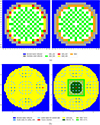Fig. 2. 2D cross section at mid-plane of the differents cores. (a) UAM-UOX (left) and UAM-MOX (right). (b) UH1.4 (left) and UMZONE (right).

3.2.2. The UH1.4 and UMZONE mock-up experiments

The experimental configurations used in this paper are the UH1.4 and UMZONE (UMZ) configurations of the EPICURE program [39] held in the EOLE critical facility [40] at CEA Cadarache in France in the nineties. This program aimed at designing critical experiments whose purpose was the validation of calculation codes for PWR-type cores with mixed UO₂/PuO₂ loadings. Measurements include critical size determination, fuel and absorber reactivity effects, as well as pin-by-pin fission rate axial and radial distributions.

UH1.4 consists of 1256 UOX-type fuel pins enriched at 3.7% and 109 guide tubes including 17 for safety, disposed in a 1 meter high and almost 1 meter radius core. “1.4” stands for the average lattice moderation ratio (additional aluminum overclad of adequate thickness surrounding the fuel pins simulates the moderation ratio of a PWR in HFP conditions).

The UMZONE configuration contains a little more UOX fuels (1264) surrounding a central threezoned 17×17 array of MOX rods with different plutonium contents (4.3%, 7% and 8.7% from periphery to center).

Both operate at ambient conditions. Figure 2b shows a 2D radial cross section at core mid-plane of the different configurations.

Two variables have been selected in our study, in order to analyse the similarity (representativity) between the industrial cores and the experiments: the effective multiplication factor (k_eff) as a global observable, and the center over periphery fission rate ratio as a local observable. As previously said, this last parameter was not initialy designed to be representative of a large reactor.

3.2.3. Uncertainty and representativity study on the effective multiplication factor

The study of the main contributors to the k_eff uncertainty reveals that a very limited number of reactions account for the majority of the uncertainty in each case (see Tab. 9 for the situation at zero power). However, the ranking is likely to evolve with the fuel cycle⁸ (see Figs. 3 and 4) as the isotopic concentrations change: the most influential isotopes at the beginning are not necessarily the same at the end.

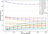Fig. 3. Distribution of the keff uncertainty over the main contributors function of the burnup at HFP: UAM-UOX.

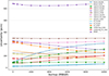Fig. 4. Distribution of the keff uncertainty over the main contributors function of the burnup at HFP: UAM-MOX.

For example, U235 reactions are progressively replaced by Pu reactions, contributing to a decrease then a stabilisation in the final uncertainty as Pu isotopes are produced and also burned. It is also very interesting to note the significant contribution of ${}_{}{}^{135}\mathrm{Xe}$ (fission product) to the final uncertainty (≳200 pcm), the value of which remains quite stable due to an evolution in equilibrium with the power level.

As regard the representativity of UH1.4 to the different cores, starting from 0.74 and 0.68 at HZP respectively (see Tab. 10), it drops due to a change in the sensitivity profiles throughout the cycle: at the beginning, the different cores, mainly loaded with UO₂ fuel presents a relatively low but satisfactory degree of similarity with UH1.4. However, as the fuel evolves⁹, the uranium isotopes are consumed while other isotopes, especially plutonium isotopes are produced leading to a differentiation in terms of sensitivity profiles and therefore, a degraded degree of similarity with the experiment (see Fig. 5).

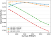Fig. 5. keff representativity function of the burnup at HFP.

In addition, we can observe a better representativity factor between the UAM cores than those of each core to UH1.4. The ambient operating conditions, the size difference between the mock-up and the core and finally the enrichment level could reasonably be pointed out to explain such a difference. However, it has been shown by varying the $B_z^2$ coefficient (and thus the leakage), the fuel and moderator temperatures, that the fuel enrichment accounts as the main parameter explaining this representativity difference, the others accounting in less proportion. This is in agreement with the analysis made in Section 3.1.3.

The same analysis is made with UMZONE and its central MOX assembly, which representativity remains at higher values due to plutonium production throughout the cycle, hence increasing the importance of the plutonium isotopes to the representativity. However, the global representativity remains low (<0.7) as the sensitivity profiles are relatively different (mainly driven by uranium and, to a lower extend, gadolinium isotopes – at least up to 12–15 GWd/T).

3.2.4. Uncertainty and representativity study on the center over periphery fission rate ratio

In the reactor cases, the fission rates are integrated over all the fuel pins of the central assembly on the one hand and of the peripheral assembly in the other (respectively at position J9 and R15 in Fig. 2a). The central assembly contains uranium-gadolinium pins while the peripheral doesn’t. They are pin-wise in the ZPR experiments cases due to their smaller size¹⁰.

Figure 6 shows the fission rate ratio function of the burnup for the various UAM cores and is completed in Appendix A with the 2D power maps of the different cores. The displacement of the hot spot and the evolution of the normalized (to the mean) assembly powers can then be observed.

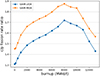Fig. 6. Fission rate ratio function of the burnup at HFP.

Unlike the k_eff, the UH1.4 is not representative of the UAM Gen-III cores (see Tab. 11) for the fission rate ratio. The size, at the first order but also the reflector type explain this lack of representativity. In the experiments, the fuel is surrounded by a large borated water layer, moderating neutrons, while the UAM cores contain a stainless steel heavy reflector that reflect neutrons in a slightly harder spectrum, hence exacerbating, through a higher reflector saving, the actual size of the core. These conceptual differences affect the shape of the power map and therefore the local fission rate ratios. However, UMZONE presents a much better representativity to UAM-MOX (–0.6).

Moreover, the negative signs indicate anti-correlations (in the sense of nuclear data) between the sensitivity profiles. Here also, the representativity factor evolves with the burnup (see Fig. 7).

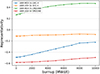Fig. 7. Fission rate ratio representativity function of the burnup at HFP.

Before suggesting an interpretation of the results, we have taken the analysis a step further by looking at the respective contributions of direct and indirect effects. Since only the isotopic fission cross-sections are concerned by the direct effect in this specific case (see Eq. 12), the comparison have concerned only the main fissile isotopes. Table 12 shows the respective relative contributions of the direct and indirect terms to the sensitivity of the total fission rate ratio at zero power. We note the difference between the mock-up experiments and the large cores. In the later case, the predominance of the indirect term indicates that a change in the flux will be more influential that the direct impact of the perturbation on the fission rate ratio. It is an indicator of a size effect on the sensitivities.

Table 13 gives the uncertainty of the center over periphery fission rate ratio and its distribution over the main contributors at zero power. With regard to the magnitude, we note the very high value of the uncertainty in the case of UAM-MOX (more than 18%). Various reactions account for the main contributors depending on the configurations.

This size effect also explains the gap between the uncertainties of mock-up experiments and those of large cores as the direct terms are generally of the same order of magnitude. In fact, the indirect effect (and therefore the influence of the immediate environment) on the fission rate ratio sensitivities results in a greater sensitivity the greater the center-periphery distance, and consequently a higher uncertainty in the case of large cores. It could indicates a greater compensation between the center and the periphery for the mock-up experiments due to their small size.

For the difference between the UOX and the MOX cores, the following interpretation can be made: the presence of the MOX assemblies in the last ring of the UAM-MOX core is responsible of a higher uncertainty. In fact, if we look at the main contributors for example, in the UAM-UOX case, a change in the U235 cross-sections will affect the immediate environment of both the central and the peripheral assemblie as they are U235 enriched assemblies and surrounded by UOX and UGD type assemblies. Thus, a variation in the central fission rate is partly compensated by a variation in the peripheral fission rate in terms of sensitivities with respect to the U235 cross-sections. A contrario, in the UAM-MOX case, the periphery contains MOX and also have MOX in its immediate environment which are less affected by a perturbation in the U235 cross-sections. Thus, a perturbation in the U235 cross-sections will lead to a less flat power map, and then a more sensitive center/periphery fission rate ratio, i.e. a larger uncertainty with respect to the input perurbation. As the fuel evolves, the uncertainty is reduced (see Figs. 8 and 9).

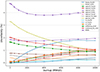Fig. 8. Distribution of the fission rate ratio uncertainty over the main contributors function of the burnup at HFP: UAM-UOX.

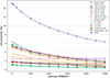Fig. 9. Distribution of the fission rate ratio uncertainty over the main contributors function of the burnup at HFP: UAM-MOX.

4. Conclusions

This paper presents a first application of experimental results issued from ZPR experiments to an advanced Gen-III core design core, based on representativity and transposition approach. After a short reminder of the mathematical background based on a deterministic bayesian inference, sensitivities are calculated using the different perturbation theories implemented in the COCAGNE deterministic core code developed by EDF and FRAMATOME, and uncertainties are propagated by the “sandwich rule”. This paper studies an application of the representativity evaluation between two Gen-III PWR cores, issued from the benchmark UAM, using the transferable information from two mock-up experiments performed in the EOLE critical facility.

The primary objective of the mock-up experiments is to produce experimental data used for the validation of calculation tools for neutron physics. They also offer a highly precise measurements database which can be used in a transposition approach in a context of complementary validation process for new reactor concepts. Then, the question was how does this representativity evolve with the configurations and during the cycle and how small cores can be representative of a large core power distribution.

Covariance data were collapsed from a fine 36-group mesh to a coarser 8-group energetic mesh according to different conservation principles: reaction rates and total uncertainties. Without ruling on the appropriateness of using one or the other, it is important to note that the variance-covariance distribution inside the fine mesh can hide a sudden jump from one group to another, from a few dozen to a few percent, for example. This seems to lead to an underestimation of progaged uncertainty when collapsing with the sensitivity profiles. Therefore, the choice of the coarse mesh with regards to the fine energy mesh bounds is important.

As a result, the first selection of well documented experiments from the EPICURE program in the EOLE ZPR showed different behaviours, according to the considered output:

• The representativities on the effective multiplication factor are relatively good and confirm that mock-up experiments are relevant for large Gen-III cores even with the presence of UO2-Gd2O3 assemblies and a stainless steel reflector.

• As for the fission rate ratio, the representativities are lower and are explained by the difference in the sizes (already pointed out by [41]) to which is added the impact of the stainless steel heavy reflector, both contributing to the neutron decoupling between the center and the periphery. However, this result doesn’t represent a drawback for the mock-up experiments, which were not originally designed to validate the power distributions of a large core, but to validate local fission rate distributions at the assembly scale.

One way to increase this representativities would be to integrate other ZPR experiments such as CAMELEON [42] (UO₂ with gadolinium pins) and PERLE [43] (UO₂ surrounded by a thick stainless steel reflector) in the ZPR database both for k_eff and for fission rate distributions, and experiments from NPP (Nuclear Power Plant) fleet especially for fission rate distributions.

Moreover, this preliminary analysis already points out several important sources of uncertainties on both k_eff and fission rate distributions. Among the main nuclear data driving the uncertainties, we can already mention ${}_{}{}^{135}\mathrm{Xe}$ capture cross-section for k_eff.

The full transposition analysis, to be published in a forthcoming paper will give potential improvements in the cross-sections for Gen-III core physics. We will highlight the potential gain of combining various experiments in ZPRs, known for their preciseness, with physical test experiments (to avoid burnup calculation biases in particular) from the french NPP fleet, less precise but more representative in particular for fission rate distributions. The combined approach of such dual experimental database, coupled with a weighting technique, enables an optimized transposition to some targeted design.

Finally, it should be noted that the UAM-MOX core is an “exotic” configuration, not representative of a possible mixed loading pattern, and has been designed only to exacerbate the effect of some nuclear data from a numerical point of view. This explains the large fission rate ratio uncertainty we observed.

Acknowledgments

The authors also want to thank Dr. Xavier Hubert from FRAMATOME for the proofreading of this paper and his relevant remarks.

Funding

This work was done under a “CIFRE” PhD grant from the french ANRT (Association Nationale Recherche Technologie – Ministry of Higher Education and Research) and conducted in the EDF Lab Paris-Saclay facility.

Conflicts of interest

The authors declare that they have no competing interests to report.

Data availability statement

The authors confirm that the associated data of this review are available within the article and online ressources in the references section.

Author contribution statement

All the authors gave important contributions to this paper. The individual contributions to this article can be summarized as follow: − E. Njayou: Data elaboration, simulations, formal analysis, writing – original draft. − P. Blaise, D. Couyras, J.-P. Argaud, L. Clouvel, N. Dos Santos: formal analysis, supervision, writing – review & editing.

References

Appendix A Normalized 2D power maps of the UAM UOX and MOX cores at various burnups.

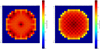Fig. A.1. Normalized 2D power map of the UAM-UOX core at 0 (left) and 4000 MWd/t (right).

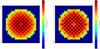Fig. A.2. Normalized 2D power map of the UAM-UOX core at 8000 (left) and 12000 MWd/t (right).

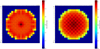Fig. A.3. Normalized 2D power map of the UAM-MOX core at 0 (left) and 4000 MWd/t (right).

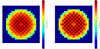Fig. A.4. Normalized 2D power map of the UAM-MOX core at 8000 (left) and 12000 MWd/t (right).

All Tables

All Figures

	Fig. 1. Some UAM GEN-III fuel assemblies.
In the text

	Fig. 2. 2D cross section at mid-plane of the differents cores. (a) UAM-UOX (left) and UAM-MOX (right). (b) UH1.4 (left) and UMZONE (right).
In the text

	Fig. 3. Distribution of the keff uncertainty over the main contributors function of the burnup at HFP: UAM-UOX.
In the text

	Fig. 4. Distribution of the keff uncertainty over the main contributors function of the burnup at HFP: UAM-MOX.
In the text

	Fig. 5. keff representativity function of the burnup at HFP.
In the text

	Fig. 6. Fission rate ratio function of the burnup at HFP.
In the text

	Fig. 7. Fission rate ratio representativity function of the burnup at HFP.
In the text

	Fig. 8. Distribution of the fission rate ratio uncertainty over the main contributors function of the burnup at HFP: UAM-UOX.
In the text

	Fig. 9. Distribution of the fission rate ratio uncertainty over the main contributors function of the burnup at HFP: UAM-MOX.
In the text

	Fig. A.1. Normalized 2D power map of the UAM-UOX core at 0 (left) and 4000 MWd/t (right).
In the text

	Fig. A.2. Normalized 2D power map of the UAM-UOX core at 8000 (left) and 12000 MWd/t (right).
In the text

	Fig. A.3. Normalized 2D power map of the UAM-MOX core at 0 (left) and 4000 MWd/t (right).
In the text

	Fig. A.4. Normalized 2D power map of the UAM-MOX core at 8000 (left) and 12000 MWd/t (right).
In the text

References

- ASN, Qualification des outils de calcul scientifique utilisés dans la démonstration de sûreté nucléaire – 1re barrière, 07. 2017 [Google Scholar]
- A. Gandini, On transposition of experimental reactor data to reference design, Technical report, Comitato nazionale per la ricerca e per lo sviluppo dell’energia nucleare e delle energie alternative (1983) [Google Scholar]
- A. Gandini, Extended bias-factor data transposition method, Trans. Am. Nucl. Soc. 50, 11 (1985) [Google Scholar]
- P. Blaise, S. Cathalau, P. Fougeras, An application of sensitivity and representativity approach for the design of a 100% MOX BWR experimental program in ZPR, Ann. Nucl. Energy 163, 108566 (2021) [CrossRef] [Google Scholar]
- N. Dos Santos, P. Blaise, A. Santamarina, A global approach of the representativity concept: application on a high-conversion light water reactor MOX lattice case, in International Conference on Mathematics and Computational Methods Applied to Nuclear Science & Engineering (M&C 2013) (Sun Valley, Idaho, USA, American Nuclear Society, LaGrange Park, IL, 2013), Vol. 5 [Google Scholar]
- G. Palmiotti, M. Salvatores, G. Aliberti, H. Hiruta, R. McKnight, P. Oblozinsky, W.S. Yang, A global approach to the physics validation of simulation codes for future nuclear systems, Ann. Nucl. Energy 36, 355 (2009) [CrossRef] [Google Scholar]
- M. Salvatores, G. Aliberti, G. Palmiotti, D. Rochman, P. Oblozinsky, M. Hermann, P. Talou, T. Kawano, L. Leal, A. Koning, I. Kodeli, Nuclear data needs for advanced reactor systems: a NEA Nuclear Science Committee initiative, in International Conference on Nuclear Data for Science and Technology (2007) [Google Scholar]
- P. Lopez, A. Bidaud, Bayesian transposition: a practical approach using nuclear reactor start up data, in ANS Winter Meeting (2021), pp. 942–945 [Google Scholar]
- V. Vallet, C. Vaglio-Gaudard, C. Carmouze, Application of the bias transposition method on PWR decay heat calculations with the DARWIN2.3 package, in GLOBAL 2017 International Nuclear Fuel Cycle Conference (Seoul, South Korea, 2017) [Google Scholar]
- K. Ivanov, M. Avramova, Benchmarks for Uncertainty Analysis in Modelling (UAM) for the Design, Operation and Safety Analysis of LWRs – Volume I: Specification and Support Data for Neutronics Cases (Phase I) (OECD Publishing, Paris, 2013) [Google Scholar]
- L.N. Usachev, Equation for the value of neutrons, reactor kinetics and perturbation theory, in Proceedings of International Conference on Peaceful Uses of Nuclear Energy (1955) [Google Scholar]
- M. L. Williams, Perturbation Theory for Reactor Analysis, CRC Handbook of Nuclear Reactor Calculations (CRC Press, 1986) [Google Scholar]
- A. Gandini, A generalized perturbation method for bi-linear functionals of the real and adjoint fluxes, Sov. At. Energy 20, 755 (1967) [Google Scholar]
- L.N. Usachev, Perturbation theory for the breeding factor, and other ratios of a number of different processes in a reactor, Sov. At. Energy 15, 1255 (1963) [CrossRef] [Google Scholar]
- A. Calloo, COCAGNE: EDF new neutronic core code for ANDROMEDE calculation chain, in Int. Conf. on Mathematics and Computational Methods Applied to Nuclear Science and Engineering (M&C) (Jeju, Korea, April 2017) [Google Scholar]
- E.M. Gelbard, Simplified spherical harmonics equations and their use in shielding problems, in ANS Winter Meeting (San Francisco, California, Dec. 1960), https://www.osti.gov/biblio/4809517 [Google Scholar]
- C. de Saint-Jean, P. Archier, B. Habert, D. Bernard, G. Noguere, J. Tommasi, P. Blaise, E. Dupont, M. Ishikawa, K. Sugino et al., Assessment of Existing Nuclear Data Adjustment Methodologies. A report by the Working Party on International Evaluation Co-operation of the NEA Nuclear Science Committee-Intermediate Report (2011) [Google Scholar]
- D. Siefman, M. Hursin, D. Rochman, S. Pelloni, A. Pautz, Stochastic vs. sensitivity-based integral parameter and nuclear data adjustments, Eur. Phys. J. Plus 133, 429 (2018) [Google Scholar]
- C.R. Rao, Linear statistical inference and its applications, Volume 2 (Wiley, New York, 1973) [CrossRef] [Google Scholar]
- A. Gelman, J.-B. Carlin, H.S. Stern, D.B. Dunson, A. Vehtari, D. B. Rubin, Bayesian Data Analysis (Taylor & Francis Ltd, 2013) [Google Scholar]
- L. Clouvel, Uncertainty quantification of the fast flux calculation for a PWR vessel, Ph.D. Thesis, Université Paris Saclay (COmUE), 2019 [Google Scholar]
- V.V. Orlov, A.A. Van’Kov, A.I. Voropaev, Yu.A. Kazanskij, V.I. Matveev, V.M. Murogov, E.A. Khodarev, Problems of fast reactor physics related to breeding, At. Energy Rev. 18, 989 (1980) [Google Scholar]
- T. Frosio, T. Bonaccorsi, P. Blaise, Extension of Bayesian inference for multi-experimental and coupled problem in neutronics – a revisit of the theoretical approach, EPJ Nucl. Sci. Technol. 4, 19 (2018) [CrossRef] [EDP Sciences] [Google Scholar]
- C.R. Weisbin, E.M. Oblow, J.H. Marable, R.W. Peelle, J.L. Lucius, Application of sensitivity and uncertainty methodology to fast reactor integral experiment analysis, Nucl. Sci. Eng. 66, 307 (1978) [CrossRef] [Google Scholar]
- E. Greenspan, Sensitivity functions for uncertainty analysis, in Advances in Nuclear Science and Technology, edited by J. Lewins and M. Becker (Springer, US, 1982), Vol. 14, pp. 193–246 [CrossRef] [Google Scholar]
- D. Rochman, A. Vasiliev, H. Ferroukhi, H. Dokhane, A. Koning, How inelastic scattering stimulates nonlinear reactor core parameter behaviour, Ann. Nucl. Energy 112, 236 (2018) [CrossRef] [Google Scholar]
- R. Sanchez, J. Mondot, Z. Stankovski, A. Cossic, I. Zmijarevic, APOLLO2: a user oriented, portable, modular code for multigroup transport assembly calculations, Nucl. Sci. Eng. 100, 352 (1988) [CrossRef] [Google Scholar]
- J.-F. Vidal, O. Litaize, D. Bernard, A. Santamarina, New modelling of LWR assemblies using the APOLLO-2 code package, in Int. Conf. on Mathematics and Computational Methods Applied to Nuclear Science and Engineering (M&C) (2007) [Google Scholar]
- R. MacFarlane, D.W. Muir, R.M. Boicourt, A.C. Kahler, The NJOY nuclear data processing system, version 2012, Technical Report LA-UR-12-27079, National Los Alamos National Laboratory (LANL), 2012 [Google Scholar]
- N. Hfaiedh, A. Santamarina, Determination of the optimised SHEM mesh for neutron transport calculation, in Proceedings of International Conference on Mathematics and Computation, M&C (2005) [Google Scholar]
- L. Goldberg, J. Vujic, A. Leonard, R. Stachowski, The characteristics method in general geometry, Trans. Am. Nucl. Soc., 73, 173 (1995) [Google Scholar]
- A. Hébert, Applied Reactor Physics (Presses internationales Polytechnique, 2020) [CrossRef] [Google Scholar]
- A. Santamarina, D. Bernard, P. Blaise, M. Coste, A. Courcelle, T.D. Huynh, C. Jouanne, P. Leconte, O. Litaize, S. Mengelle, G. Noguère, J-M. Ruggiéri, O. Sérot, J. Tommasi, C. Vaglio, J-F. Vidal, The JEFF-3.1.1 Nuclear Data Library Validation Results from JEF-2.2 to JEFF-3.1.1, Technical report, Nuclear Energy Agency, 2009 [Google Scholar]
- A. Rizzo, G. Noguère, P. Tamagno, Private communication on COMAC-V2.1 identification sheet [Google Scholar]
- P. Archier, C. De Saint Jean, O. Litaize, G. Noguère, E. Privas, L. Berge, P. Tamagno, CONRAD evaluation code: development status and perspectives, Nucl. Data Sheets 118, 488 (2014) [CrossRef] [Google Scholar]
- C. De Saint Jean, P. Archier, G. Noguere, O. Litaize, C. Vaglio-Gaudard, D. Bernard, O. Leray. Estimation of multi-group cross section covariances of 235,238U, 239Pu, 241Am, 56Fe, 23Na and 27Al, in Proceedings of the PHYSOR2012 Conference, Knoxville, Tennessee, USA, 04 2012 (American Nuclear Society, LaGrange Park, IL, 2012) [Google Scholar]
- H. Hiruta, G. Palmiotti, M. Salvatores, R. ArcillaJr., P. Oblozinsky, R.D. McKnight, Few group collapsing of covariance matrix data based on a conservation principle, Nucl. Data Sheets 109, 2801 (2008) [CrossRef] [Google Scholar]
- A.J.M. Plompen et al., The joint evaluated fission and fusion nuclear data library, JEFF-3.3, Eur. Phys. J. A 56, 181 (2020) [Google Scholar]
- J. Mondot, EPICURE: an experimental program devoted to the validation of the calculational schemes for plutonium recycling in PWRs, in International Conference on the Physics of Reactors, Physor90 (Marseille, France, 1990), Vol. 121, pp. 32–40 [Google Scholar]
- P. Fougeras, S. Cathalau, J. Mondot, P. Klenov, Optimization of a calculation scheme for the treatment of plutonium recycling in pressurized water reactors, Nucl. Sci. Eng. 121, 32 (1995) [CrossRef] [Google Scholar]
- N. Dos Santos, Optimisation de l’approche de représentativité et de transposition pour la conception neutronique de programmes expérimentaux dans les maquettes critiques, Ph.D. Thesis, Université Grenoble Alpes, 2013 [Google Scholar]
- P. Blaise, O. Litaize, J.-F. Vidal, A. Santamarina, Qualification of the French APOLLO2.8/CEA2005V4 code package on absorber clusters in 17×17 PWR type lattices through the CAMELEON program, in International Conference on the Physics of Reactors, Physor2010 (Pittsburgh, 2010) [Google Scholar]
- A. Santamarina, C. Vaglio-Gaudard, P. Blaise, J.-C. Klein, N. Huot, O. Litaize, N. Thiollay, J.-F. Vidal, The PERLE experiment for the qualification of PWR heavy reflectors, in International Conference on the Physics of Reactors, Physor2008 (Interlaken, Switzerland, 2008) [Google Scholar]