| Issue |
EPJ Nuclear Sci. Technol.
Volume 2, 2016
|
|
|---|---|---|
| Article Number | 23 | |
| Number of page(s) | 10 | |
| DOI | https://doi.org/10.1051/epjn/2016011 | |
| Published online | 27 April 2016 | |
https://doi.org/10.1051/epjn/2016011
Regular Article
Thermodynamic exergy analysis for small modular reactor in nuclear hybrid energy system
1
Rensselaer Polytechnic Institute, 110 8th Street, JEC 5046, Troy, NY 12180, USA
2
Idaho National Laboratory, PO Box 1625, Idaho Falls, ID 8341, USA
⁎ e-mail: This email address is being protected from spambots. You need JavaScript enabled to view it.
Received:
5
May
2015
Accepted:
10
February
2016
Published online:
27
April
2016
Abstract
Small modular reactors (SMRs) provide a unique opportunity for future nuclear development with reduced financial risks, allowing the United States to meet growing energy demands through safe, reliable, clean air electricity generation while reducing greenhouse gas emissions and the reliance on unstable fossil fuel prices. A nuclear power plant is comprised of several complex subsystems which utilize materials from other subsystems and their surroundings. The economic utility of resources, or thermoeconomics, is extremely difficult to analyze, particularly when trying to optimize resources and costs among individual subsystems and determine prices for products. Economics and thermodynamics cannot provide this information individually. Thermoeconomics, however, provides a method of coupling the quality of energy available based on exergy and the value of this available energy – “exergetic costs”. For an SMR exergy analysis, both the physical and economic environments must be considered. The physical environment incorporates the energy, raw materials, and reference environment, where the reference environment refers to natural resources available without limit and without cost, such as air input to a boiler. The economic environment includes market influences and prices in addition to installation, operation, and maintenance costs required for production to occur. The exergetic cost or the required exergy for production may be determined by analyzing the physical environment alone. However, to optimize the system economics, this environment must be coupled with the economic environment. A balance exists between enhancing systems to improve efficiency and optimizing costs. Prior research into SMR thermodynamics has not detailed methods on improving exergetic costs for an SMR coupled with storage technologies and renewable energy such as wind or solar in a hybrid energy system. This process requires balancing technological efficiencies and economics to demonstrate financially competitive systems. This paper aims to explore the use of exergy analysis methods to estimate and optimize SMR resources and costs for individual subsystems, based on thermodynamic principles – resource utilization and efficiency. The paper will present background information on exergy theory; identify the core subsystems in an SMR plant coupled with storage systems in support of renewable energy and hydrogen production; perform a thermodynamic exergy analysis; determine the cost allocation among these subsystems; and calculate unit exergetic costs, unit exergoeconomic costs, and first and second law efficiencies. Exergetic and exergoeconomic costs ultimately determine how individual subsystems contribute to overall profitability and how efficiencies and consumption may be optimized to improve profitability, making SMRs more competitive with other generation technologies.
© L. Boldon et al., published by EDP Sciences, 2016
 This is an Open Access article distributed under the terms of the Creative Commons Attribution License (http://creativecommons.org/licenses/by/4.0), which permits unrestricted use, distribution, and reproduction in any medium, provided the original work is properly cited.
1 Introduction
To assess the inherent value of energy in a thermal system, it is necessary to understand both the quantity and quality of energy available or the exergy. Exergy represents the quality of energy by incorporating the actual energy available to perform work through reversible processes up to the point at which thermodynamic equilibrium with the surroundings is reached. It is the useful work potential in a system [1–4]. Not all energy is created equal, which is why assessing its quality through an exergy analysis is more revealing than simply analyzing energy.
Exergy analysis applications have expanded and often incorporate costs, providing thermoeconomic information on each component within a system. This requires converting economic costs to exergetic costs, allowing for a comparison which was previously not possible. Ultimately, this may be used to determine how individual components contribute to overall system efficiencies and costs and may even help optimize the system. This type of study cannot be performed looking at energy efficiencies alone, as these do not appropriately allocate the costs between different components, subsystems, or streams. Exergy, however, provides information on the true value of the inputs and outputs of a component. In general, a thermodynamic analysis determines a performance criteria or metric for a particular system or uses energy balances to determine where losses are occurring [1]. The former approach is not always useful, as there may be no telling metric; the latter approach neglects differences in energy quality – or considers distinct types of energy as equivalent. The results tend to not include internal losses [1].
Valero and Torres detailed the process of performing a thermoeconomic exergy analysis as a potential method of diagnosing and optimizing thermal energy systems [2]. It may also be used to help determine appropriate prices for any products made by the plant based on thermodynamic properties; to optimize a particular portion of the system in an effort to reduce operating or production costs; to identify inefficiencies and their resulting effects on resource consumption or system economics; and to compare different design features or options [2,3].
In general, exergy analyses are useful in studying potential energy savings, recognizing that the theoretical savings will always be higher than the actual savings enacted as a result of constraints imposed by operational, etc. decisions or limits [5,6].
The thermoeconomics of power plants producing heat and/or electricity may be readily studied with an exergy analysis. This report provides relevant background information on exergy concepts, details the methodology behind an exergy analysis, and provides theoretical first and second law results for a nuclear hybrid energy system with thermal storage.
2 Exergy
The first and second laws of thermodynamics are at the foundation of exergy and provide a mechanism of comparing exergy and energy analysis results. The first law states that energy is never created or destroyed. It is simply transformed to a different form, such that the change in energy ΔE may be determined by the difference in heat added Q and work W, Q – W = ΔE [4,7]. The second law describes the creation of entropy in an energy transfer due to dissipative energy losses [7]. Understanding these fundamental principles is significant in identifying thermodynamic losses and attempting to minimize these losses.
2.1 Reversible vs. irreversible processes
A reversible process is a process in which properties such as temperature may be altered without generating entropy. In such a process, there is no change to the system or its surroundings. On the other hand, when an irreversible process occurs, entropy increases and exergy is destroyed or reduced. In a realistic cycle, there will always be some irreversibilities or losses, and equation (1) may be used to determine the destroyed exergy Xdestroyed per the Gouy-Stodola theorem, where Sgen is the generated entropy and T0 is the temperature of the surroundings [3]. In general, if the destroyed exergy or the generated entropy are equal to zero, the process may be considered internally reversible. If either is greater than zero, the process is irreversible. (1)
(1)
2.2 Exergy within a system
There are distinct types of exergy, including heat, chemical, and work exergy. The exergy of heat energy is dependent upon the component efficiency and the temperatures of the heat source and heat sink or surroundings. The exergy of work energy is equal, as 100% of the work can be directly utilized. Chemical reactions may produce energy, some of which may be turned into heat or other forms. Only a fraction of the chemical energy is exergy. This article focuses on heat and work exergy in nuclear power plant flows.
For a system of heat and work flows, the change in system exergy ΔXsystem may be calculated from equation (2), where ΔXheat, Xwork, and Xdestroyed represent the change in heat exergy and the work and destroyed exergy respectively. (2)
(2)
When analyzing a particular system, it is necessary to identify the flows in and out of the system and to determine whether the system should be treated as closed or open. To do this, the system boundary and surroundings must be identified. In a closed system, mass is not permitted to pass the boundary and the mass is fixed; only energy may pass the boundary and interact with the surroundings. In an open system, both mass and exergy are permitted to flow through the system boundary. An isolated system is a closed system in which neither energy nor mass crosses the system boundary.
Calculating the exergy balance for both closed and open systems requires understanding the energy and entropy balances as the system progresses from state 1 to state 2, as shown in equations (3) and (4), where Q represents heat added or rejected, W represents work, E is energy, and S is entropy.  for an adiabatic system. If the temperature of Q is not constant, then
  .
. (3)
(3)
 (4)
(4)
The energy at each state E1 and E2 may be calculated from the respective internal, potential, and kinetic energies.
Equation (5) shows internal energy U based upon enthalpy H, pressure P, and volume V. Equations (6) and (7) show the exergies at each state. The exergy for each state for unit mass may be calculated by equations (8) and (9). (5)
(5)
 (6)
(6)
 (7)
(7)
 (8)
(8)
 (9)
(9)
The change in exergy for the system may then be determined from equations (5) to (9).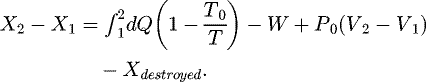 (10)
(10)
2.3 Exergy flows and transfer
Exergy transfer must also be accounted for in a system. It occurs via heat, work, or mass flows. The Carnot cycle efficiency 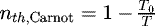 represents the max exergy or work that can be achieved from heat transfer [7]. This heat exergy is shown in equation (11), where heat added Q = cp
m (T2 – T1).
represents the max exergy or work that can be achieved from heat transfer [7]. This heat exergy is shown in equation (11), where heat added Q = cp
m (T2 – T1). (11)
(11)
It is more realistic to use the efficiency based on the power cycle being analyzed, rather than an ideal Carnot cycle. For this case, the thermal efficiency would be 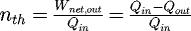 [7]. A process efficiency may be calculated as the ratio of the increase in exergy over the decrease in exergy [4]. In a thermodynamic cycle, the entire cycle efficiency may be described in the same manner, representing the second law efficiency [4].
Work exergy transfer can occur via boundary work, meaning the boundary of the system changes, such as expansion/compression in a piston/cylinder system, or via mechanical/shaft or electrical work. In the former case, only a portion of the work is completely useful, while some is lost to the surroundings, as shown in equation (12). The latter exergy transfer results in entirely useful work, such that Xmechanical = W. (12)
(12)
Mass exergy transfer occurs in an open system proportionally to the system flow rate. It has exergy, energy, and entropy, as shown in equation (13), where m represents mass. This article does not focus on mass transfer within the system analyzed.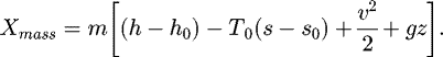 (13)
(13)
3 Methods and materials
3.1 Nuclear renewable energy integration
This article breaks down the exergy of individual components within the Nuclear Renewable Energy Integration (NREI) system shown in Figure 1, where nuclear energy is supplementing the available wind energy through storage to meet the needs of the electrical grid. Nuclear power is also being used for the production of hydrogen via high temperature steam electrolysis.
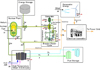 |
Fig. 1 Nuclear renewable energy integration schematic. |
3.2 System breakdown and assumptions
The process flows utilized in this analysis are also displayed in Figure 1. The following assumptions were made to analyze the system:
-
steady state operation;
-
required electrical output to grid is 245 MWe;
-
wind electric production is constant at 100 MWe with 5 MWe in frictional heat losses;
-
high temperature steam electrolysis requires 5 MWth and 1 MWe to produce 2780 Nl/min with a 50% thermal conversion efficiency [8];
-
high temperature helium-cooled small modular reactor with 300 MWth capacity;
-
compressed air energy storage is at maximum capacity of 400 MW;
-
reactor outlet temperature and pressure of 850 °C and 5 MPa [8,9];
-
average reactor fuel temperature of 1000 °C;
-
heat loss in reactor is assumed to occur from heat transfer inefficiencies from fuel to helium;
-
generator exhibits 1% heat losses [10];
-
turbine isentropic efficiency of 89% [11];
-
compressor isentropic efficiency of 86% [11];
-
no electric losses incurred during high temperature steam electrolysis (HTSE);
-
losses incurred in the low temperature heat exchanger are not considered;
-
constant pressure across heat exchanger;
-
4% frictional pressure drop in turbine [11].
A closed Brayton power cycle with helium was used in this analysis, as shown in Figure 2. The overall Brayton cycle efficiency is a function of the work in and out of the system and the heat added to the system, as shown in equation (14). The turbine will turn the shaft which powers the compressor and generator. Since the compressor will use a substantial amount of the turbine work/power, it is necessary to determine fraction of work, or backwork ratio (BW), to the compressor using equation (15). The generator then sees (1 – BW) × Turbine Output. (14)
(14)
 (15)
(15)
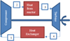 |
Fig. 2 NREI Brayton power cycle. |
3.3 Resources, products, and losses
To properly identify the production function for a unit and how the unit contributes to the plant function, it is necessary to define each unit's product (P), resources (F), and losses (L) and identify which flows they correspond to [3]. In other words, the production function may be determined by using the F-P-L definition, such that every flow into or out of a unit is incorporated once; every component has an overall exergy greater than or equal to zero; and the exergy balance for each unit follows the form F – P – L = D, where D refers to exergy destruction or unavoidable losses [3]. The total irreversibility then becomes the sum of the process losses and exergy destruction I = F – P = L + D. Table 1 shows the distribution of flows amongst resources, products, and losses based on unit and for the entire plant.
Once again following the F-P-L definition yields the matrix M = MF – MP – ML, as shown in Table 2. The individual incidence matrices for resources, products, and losses were derived from Table 1, where the respective flows are shown, along with a positive or negative sign indicating whether the flow adds or subtracts from the unit's exergy.
Unit flow distribution of resources, products, and losses.
F-P-L incidence matrix for NREI system.
3.4 Exergetic cost of flows
The exergetic cost  (MW) may be defined as the necessary exergy for a process or flow. It provides a method for comparing units or components producing different quality products – for example, heat vs. electrical work – and also helps bridge the gap between plant thermodynamics and economics. The unit exergetic cost
  is simply the ratio of the exergetic cost to the exergy Xi, or
  [2,3].
Several propositions have been developed based on energy/exergy relationships within a thermal system, so that the system of cost allocation equations may be determined, thereby allowing one to solve for the exergetic costs for each component and the entire plant [3,12]:
-
the exergetic cost for each unit may be considered conservative;
-
the exergetic cost for the plant flows may be equated with the exergy of the flow;
-
exergetic cost of losses is assumed to be zero when no external assessment or influence is made;
-
in the case where a flow is both an output and an input to a unit, the unit exergetic costs are considered equal. In the case where the output of a unit consists of several flows, the unit exergetic cost of each output flow is considered equal.
The first proposition states that the exergy balance for each unit must equal zero, or M × X* = 0, where X* is a [23 × 1] matrix containing all the unknown exergetic cost values  for each flow i. The second proposition relates the plant inputs to their respective exergies, such that the exergetic cost of each input may be equated to its exergy,
  , where j represents plant. The third proposition makes an assumption about the value of the losses, such that Xk,losses = 0, where k represents individual subsystems or units. The fourth and final proposition refers to two separate cases, one in which the unit exergetic costs are equivalent for a subsystem yielding two products,
  , and the other when a flow is both input and output for a particular subsystem,
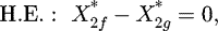
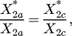
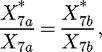
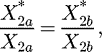
  [2]. These propositions provide a system of 23 equations, which are presented in equations (16) to (33) with their respective proposition indicated:
-
Proposition 1:
 (16)
(16)
 (17)
(17)
 (18)
(18)
 (19)
(19)
 (20)
(20)
 (21)
(21)
 (22)
(22)
-
Proposition 2 (Plant):
 (23)
(23)
 (24)
(24)
 (25)
(25)
 (26)
(26)
-
Proposition 3 (Losses):
 (27)
(27)
-
Proposition 4:
-
product of multiple flows:
 (28)
(28)
 (29)
(29)
 (30)
(30)
 (31)
(31)
-
output is also input to subsystem:
 (32)
(32)
 (33)
(33)
-
Unit exergy consumption refers to the resource exergy consumed or used within the subsystem to yield the subsystem product [2,3]. First and second law subsystem efficiencies and unit consumption may be calculated from  ,
,  , and
, and  , respectively, where XF,
  , and
, and  refer to the resource exergy, exergetic cost, and unit exergetic cost and XP,
  , and
, and  refer to the product exergy, exergetic cost, and unit exergetic cost. The total irreversibilities within each subsystem are also a function of the resources and products, Ii = XF,i – XP,i [2,3].
3.5 Exergoeconomic cost of flows
The final stage in a thermoeconomic analysis requires incorporating economic market conditions, such as the costs associated with resources and operations. This yields the exergoeconomic cost ($/s), or rather the money required to create the previously detailed flows in the system [2]. The amortized cost rate ($/s) of installation and operations for each subsystem Zi must be determined, such that a system of equations may be developed based on the cost balance shown in equation (34), where ci represents the unit exergoeconomic cost of a product or resource ($/MW × s) [2,3]. Any losses are assumed to have a cost of zero. The exergoeconomic cost is then Ci = ci
Xi. (34)
(34)
The cost balance equations for the NREI subsystems are shown in equations (35) to (41).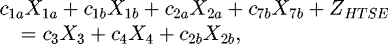 (35)
(35)
 (36)
(36)
 (37)
(37)
 (38)
(38)
 (39)
(39)
 (40)
(40)
 (41)
(41)
Most of the subsystems have more than one input and/or output, so the cost balance equations do not provide enough information to solve for the unit exergoeconomic costs. It is therefore necessary to make assumptions regarding the importance of plant products. The extraction method is used in this analysis, such that the priority is assigned to electricity production, which will bear the system's overall costs [2]. This is deemed reasonable, as only 5 MWth is utilized for hydrogen production and is negligible compared to the electric generation costs. The unit exergoeconomic cost for a subsystem's product that is not related to electricity production will equal its unit exergoeconomic cost input, or c2a = c1c. Several plant inputs (water, air, and wind) are considered free, thus c1a = c1b = c1d = 0. The fuel cost may be estimated by  , because fuel makes up approximately 31% of nuclear power plant operation and maintenance costs, which are assumed to account for half of the installation and operation costs [13]. The exergoeconomic cost of storage will be equivalent to the energy storage installation and operation cost rate, c2e
X2e = Zstorage. The electricity produced will have the same unit exergoeconomic cost as will the hydrogen and oxygen flows, such that c7a = c7b and c3 = c4.
, because fuel makes up approximately 31% of nuclear power plant operation and maintenance costs, which are assumed to account for half of the installation and operation costs [13]. The exergoeconomic cost of storage will be equivalent to the energy storage installation and operation cost rate, c2e
X2e = Zstorage. The electricity produced will have the same unit exergoeconomic cost as will the hydrogen and oxygen flows, such that c7a = c7b and c3 = c4.
4 Results and discussion
4.1 Brayton cycle and thermodynamic properties
The T-s diagram in Figure 3 illustrates the thermodynamic properties of the NREI system, which are displayed in Table 3.
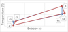 |
Fig. 3 T-s diagram (isentropic in blue and actual in red). |
Thermodynamic properties of Brayton cycle.
4.2 Energy, exergy, and exergetic cost of flows
Table 4 displays the energy, exergy, and unit exergetic cost of the flows. There are several flows into the plant, such as air or water, which are considered limitless, so the energy is set to zero, meaning there is no exergetic cost for these products. The energy for other flows refers to the power (MW), while the exergy is the power available as a result of irreversibilities – both unavoidable heat losses and process efficiency losses. Flows 5 and 6 represent the mechanical work produced by the turbine, which must turn the shaft for the compressor and generator. A backwork ratio of 54.4% was determined from equation (15) using the required input and output work to the cycle.
The reactor losses, flow 10, were calculated from the reactor efficiency  , where hmax and hHe represent the enthalpies of helium at the fuel and reactor outlet temperatures, respectively. The other heat losses were determined as a function of component efficiencies and cycle loss assumptions. For example, helium expands in the turbine from state 3 to state 4 in Figures 2 and 3 (or state 4s in an isentropic Brayton cycle).
The losses may be calculated from wturb,loss = h4a – h4s, where  and
and  represents the turbine isentropic efficiency. Similarly, the compressor losses are wcomp,loss = h2a – h2s. The exergy of all heat losses is zero. The exergy of hydrogen and oxygen were also set to 0.5 MW or half of the resultant energy (50% efficient process) [8]. The energy values for the helium flows were all determined based on what was available from the reactor after hydrogen production, respective component efficiencies, and the energy demand from the substation. In general, the exergy is then simple to determine for heat and work flows,
  , where Ej is the flow energy, T0 is the reference temperature of the surroundings (25 °C), and Tj is the flow temperature [3].
NREI component conditions (MW).
4.3 Subsystem resource exergy consumption, efficiencies, and irreversibilities
The exergy of the resources and products of individual subsystems may be determined from the exergy of each flow, as shown in Table 5. The resource/product exergy and exergetic cost were calculated by summing the exergy and exergetic cost flows, respectively, from Table 4 in the manner shown in Table 1. The first law or energy efficiency is also included in Table 5, to better demonstrate where improvements could be made to enhance the system performance [2,3]. Systems with very high second law or exergy efficiencies have limited room for improvement, as the majority of irreversibilities are unavoidable losses due to exergy destruction. This is not always clear from the first law efficiency, as in the case of the SMR, where the second law efficiency is quite high at 93.3%, while the first law efficiency is 81.5%. Similarly, the difference between the first and second law efficiencies for the HTSE demonstrates how there is less work potential than anticipated from the first law efficiency. Some systems, like the heat exchanger, see a very high first law efficiency and a low second law efficiency, illustrating how the magnitude of energy lost is very small compared to the input energy, but the lost energy is useful work potential not captured by the turbine.
Subsystem resource and product energy and exergy (MW), consumption, irreversibilities (MW), and efficiencies.
4.4 Exergoeconomics and optimization
Using the following example installation/operation cost rates and equations (35) to (41) yields the unit exergoeconomic costs for the product flows shown in Table 6: ZHTSE = $0.06/s, ZSMR = $0.30/s, Zturb = $0.06/s, ZHE = $0.003/s, Zcomp = $0.04/s, ZGen = $0.003/s, ZWind = $0.20/s, and c2e = Zstorage = $0.03/s.
An optimized thermoeconomic analysis of the NREI system would require setting additional constraints and determining an appropriate function to optimize [2]. To optimize costs, or more specifically the levelized cost to create the products, the objective function may follow the form,  , where ce and Xe are the cost and exergy for resources external to the system [2]. Incorporating possible subsystem efficiency improvements and mathematically iterating would provide a method of optimizing the exergoeconomic costs for NREI.
Tsatsaronis and Moran described how complex systems, such as NREI, may be difficult to optimize using typical mathematical models, due to lack of information on individual components – particularly if they are purchased, computational time, and possible changes to the overall system structure that may be much more profitable than the initial design [14]. A mathematical model would not be able to consciously make these structural changes. Manually iterating based on possible changes to temperature, turbine/compressor pressure ratios and efficiencies, etc. provides a better understanding of the system at hand, and for increasingly complex systems, may be a more effective manner of balancing exergy and costs [14].
Unit exergoeconomic costs.
5 Conclusion
A thermoeconomic study of an energy system provides significant information on how the system operates on both a technical – efficiencies and losses – and economic level. The coupling of these two fields through exergy and exergoeconomic analyses offers insight into methods of improving the economic competitiveness of complex systems incorporating advanced small modular reactors, energy storage, hydrogen production, and renewable energy technologies, all of which serve to meet escalating energy demands in a sustainable manner. This paper details relevant exergy concepts, explores how exergy and exergoeconomic analyses could be beneficial in assessing the Nuclear Renewable Energy Integrated system, and provides theoretical first and second law efficiencies, exergetic costs, and exergoeconomic costs for this example system.
Acknowledgments
We would like to thank the DOE for its support through the Nuclear Energy University Program Graduate Fellowship. Any opinions, findings, conclusions or recommendations expressed are those of the authors and do not necessarily reflect the view of the Department of Energy Office of Nuclear Energy or Idaho National Laboratory.
Nomenclature
BC: Brayton cycle
BW: backwork ratio
η : efficiency
E : energy/power (MW)
h : enthalpy (kJ/kg)
s : entropy
Sgen : entropy generated
X* : exergetic cost (MW)
C : exergoeconomic cost ($/s)
X : exergy (MW)
D, Xdestroyed : exergy destruction (MW)
q, Q : heat added
Z : installation and operation cost rate ($/s)
H.E.: heat exchanger
HTSE: high temperature steam electrolysis
I : irreversibility (MW)
L : losses (MW)
MJ, MW: mega-Joule, mega-Watt
NREI: nuclear renewable energy integration
P, P0 : pressure, reference pressure (101.4 kPa)
P, F : product or resource (subscript)
k : resource consumption
SMR: small modular reactor
T, T0 : temperature, reference temperature (25 °C)
W : work
k*: unit exergetic cost (MW/MW)
c : unit exergoeconomic cost ($/MJ)
References
- T.J. Kotas, The exergy method of thermal plant analysis (Department of Mechanical Engineering, Queen Mary and Westfield College, University of London, UK, 1995) [Google Scholar]
- A. Valero, C. Torres, Thermoeconomic analysis, Center of Research for Energy Resources and Consumption, Centro Politecnico Superior, Universidad de Zaragoza, Spain [Google Scholar]
- M.A. Lozano, A. Valero, Theory of the exergetic cost, Energy 18 , 939 (1993) [CrossRef] [Google Scholar]
- D. Abata, Exergy, in The Concept of Exergy (2011), Chap. 8 [Google Scholar]
- P. Le Goff, Énergétique industrielle. Tome 1 : Analyse thermodynamique et mécanique des économies d’énergie (Technique et Documentation, Paris, France, 1979) [Google Scholar]
- A. Valero, Bases termoeconómicas des ahorro de energía, in 2a Conferencia national sobre ahorro energético y alternativas energéticas , Zaragoza, Spain (1982) [Google Scholar]
- D. Kaminski, M. Jensen, Introduction to thermal and fluids engineering (Wiley Publishing, 2011) [Google Scholar]
- High-temperature electrolysis unlocking hydrogen's potential with nuclear energy, Idaho National Laboratory, Document 08-GA50044-06, 2005 [Google Scholar]
- Q. Zhang, H. Yoshikawa, H. Ishii, H. Shimoda, Thermodynamic and economic analyses of HTGR cogeneration system performance at various operating conditions for proposing optimized deployment scenarios, J. Nucl. Sci. Technol. 45 , 1316 (2008) [CrossRef] [Google Scholar]
- Efficiency in electricity generation, EURELECTRIC preservation of resources working group's upstream sub-group in collaboration with VGB, 2003 [Google Scholar]
- Gas turbines and jet engines, University of Tulsa, 2000, www.personal.utulsa.edu/∼kenneth-weston/chapter5.pdf [Google Scholar]
- A. Valero, M.A. Lozano, M. Muñoz, A general theory of exergy saving: Part I. On the exergetic cost, Part II. On the thermoeconomic cost, Part III. Exergy saving and thermoeconomics, Comput. Aided Eng. Energy Syst. 3 , 1 (1986) [Google Scholar]
- Nuclear Energy Institute, Fuel as a percent of production costs, 2013, available at: http://www.nei.org/Knowledge-Center/Nuclear-Statistics/Costs-Fuel,-Operation,-Waste-Disposal-Life-Cycle/Fuel-as-a-Percent-of-Production-Costs [Google Scholar]
- G. Tsatsaronis, M. Moran, Exergy-aided cost minimization, Energy Convers. Mgmt 38 , 1535 (1997) [CrossRef] [Google Scholar]
Cite this article as: Lauren Boldon, Piyush Sabharwall, Cristian Rabiti, Shannon M. Bragg-Sitton, Li Liu, Thermodynamic exergy analysis for small modular reactor in nuclear hybrid energy system, EPJ Nuclear Sci. Technol. 2, 23 (2016)
All Tables
Subsystem resource and product energy and exergy (MW), consumption, irreversibilities (MW), and efficiencies.
All Figures
|
Fig. 1 Nuclear renewable energy integration schematic. |
| In the text | |
|
Fig. 2 NREI Brayton power cycle. |
| In the text | |
|
Fig. 3 T-s diagram (isentropic in blue and actual in red). |
| In the text | |
Current usage metrics show cumulative count of Article Views (full-text article views including HTML views, PDF and ePub downloads, according to the available data) and Abstracts Views on Vision4Press platform.
Data correspond to usage on the plateform after 2015. The current usage metrics is available 48-96 hours after online publication and is updated daily on week days.
Initial download of the metrics may take a while.