| Issue |
EPJ Nuclear Sci. Technol.
Volume 2, 2016
|
|
|---|---|---|
| Article Number | 17 | |
| Number of page(s) | 12 | |
| DOI | https://doi.org/10.1051/epjn/e2016-50058-x | |
| Published online | 08 April 2016 | |
https://doi.org/10.1051/epjn/e2016-50058-x
Regular Article
Statistical model of global uranium resources and long-term availability
1
French Alternative Energies and Atomic Energy Commission, I-tésé, CEA/DEN, Université Paris Saclay, 91191
Gif-sur-Yvette, France
2
Université Montpellier 1–UFR d’Économie–CREDEN (Art-Dev UMR CNRS 5281), Avenue Raymond Dugrand, CS 79606, 34960
Montpellier, France
⁎ e-mail: This email address is being protected from spambots. You need JavaScript enabled to view it.
Received:
25
September
2015
Received in final form:
5
January
2016
Accepted:
19
January
2016
Published online:
8
April
2016
Abstract
Most recent studies on the long-term supply of uranium make simplistic assumptions on the available resources and their production costs. Some consider the whole uranium quantities in the Earth's crust and then estimate the production costs based on the ore grade only, disregarding the size of ore bodies and the mining techniques. Other studies consider the resources reported by countries for a given cost category, disregarding undiscovered or unreported quantities. In both cases, the resource estimations are sorted following a cost merit order. In this paper, we describe a methodology based on “geological environments”. It provides a more detailed resource estimation and it is more flexible regarding cost modelling. The global uranium resource estimation introduced in this paper results from the sum of independent resource estimations from different geological environments. A geological environment is defined by its own geographical boundaries, resource dispersion (average grade and size of ore bodies and their variance), and cost function. With this definition, uranium resources are considered within ore bodies. The deposit breakdown of resources is modelled using a bivariate statistical approach where size and grade are the two random variables. This makes resource estimates possible for individual projects. Adding up all geological environments provides a repartition of all Earth's crust resources in which ore bodies are sorted by size and grade. This subset-based estimation is convenient to model specific cost structures.
© A. Monnet et al., published by EDP Sciences, 2015
 This is an Open Access article distributed under the terms of the Creative Commons Attribution License (http://creativecommons.org/licenses/by/4.0), which permits unrestricted use, distribution, and reproduction in any medium, provided the original work is properly cited.
1 Long-term cumulative supply curves (LTCS)
The availability of natural uranium will have a direct impact on the global capability to build new nuclear reactors in the coming decades as it is forecasted that Light Water Reactors (LWRs) will remain the main nuclear technology for most of the 21st century [1,2]. The cost associated with this availability is also important. Even though its share in the electricity production cost is relatively low, it may influence the choice of fuel cycle options in the short term or the choice of reactor technologies in the long term.
1.1 Concepts and objectives
Considering natural uranium as any other mineral commodity, academics in mineral economics and decision makers in mining industries usually look at availability by the mean of two analytical tools. The first one is generally called cash-cost curve. This curve consists in plotting the cumulated production capacity (tU/year) of all known production capacities, either running mines or short-term projects, against the unit production cost ($/kgU) of those mines once they have been sorted by cost merit order. This tool essentially helps analyzing short-term to medium-term availability issues, i.e. from a couple of years to a decade or two.
Since the objective of this research is to analyze the adequacy of uranium supply to long-term demand, another tool was preferred as it suits availability problems with implications over several decades. This tool is the long-term cumulative supply curve (LTCS). It was made popular by Tilton et al. [3,4] in 1987. The curve depicts the cumulated amount (tU) of all known resources, eventually adding estimates of undiscovered resources, after they have been sorted by rising unit production cost ($/kgU). Unlike cash-cost curve, there is no time dimension in the LTCS curve. In order to assess the adequacy of supply to demand over time, one would need to compare the LTCS curve with a time-dependent demand scenario. In this paper, the stress is put on the method used to build the LTCS curve.
1.2 Aggregated LTCS curve
The easiest way to build a LTCS curve is to aggregate existing data of cumulated resources and associated production costs published in the literature or in technical reports. Focusing on uranium, this can be achieved by gathering the resources declared by countries in the IAEA/OECD-NEA biennial report called the Red Book [5]. The result is shown in Figure 1 for the aggregation of total known resources (Reasonably Assured Resources [RAR] and Inferred Resources [IR], red curve, and for total known and prognosticated resources [RAR + IR + Prognosticated Resources (PR) + Speculative Resources (SR)], light-red curve).
1.3 Limits of the aggregation approach
The aggregation approach to build LTCS curves is convenient provided that consistent data are available. Conversely, it can be criticized due to the aggregation of different levels of uncertainty in the example of the Red Book data. By definition, the amount and the cost of prognosticated or speculative resources are more uncertain than known resources (RAR or IR) to which they were added in the light-red curve (Fig. 1). While the analysis is usually performed by assuming that cheaper resources are extracted first, there is no guarantee that undiscovered resources between 40 and 80 $/kgU will all be discovered before RAR at below 80 $/kgU are exhausted. Conversely, if one only considers known resources (red curve, Fig. 1), it is likely that some resources at below 80 $/kgU that are not known at present will be discovered in the long term.
Finally, using aggregated data to perform analysis on LTCS curves has two limits. First, when data are incomplete, long-term resources are underestimated. Second, when data are over-aggregated, short-term resources may be overestimated while the long-term is affected by a growing uncertainty on costs. This appears on the upper part of the light-red curve for which 3 MtU of SR are missing since they have no cost estimate reported in the Red Book. These limits prompted some academics to develop alternative methods to build LTCS curve.
2 Global elastic crustal abundance models
To avoid aggregating estimates with different cost and amount uncertainties, some recent studies, mainly conducted by Schneider from University of Texas and Matthews and Driscoll from MIT [6–8], model the costs and quantities of resources of the entire Earth's crust with the same methodology. They introduce a 3-step method to build LTCS curves:
-
first, they model the link between the quantity (cumulated amount) and the quality (represented by ore grade) of resources;
-
second, they model the link between the unit production cost and the quality of resources;
-
finally, they infer from the first two steps the general relation between cumulated amounts of resources and associated costs.
From this framework, the elastic crustal abundance model provides a LTCS curve for the entire world.
2.1 Step 1: quantity-quality relationship
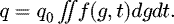
The authors introduce a power relationship between the grade g and the cumulated amount of metal q according to equation (1). This results in an elastic relationship in log-scale where α is the elasticity of quantities in relation to grades and where q0 and g0 are calibration parameters.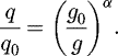 (1)
(1)
As explained in the MIT study [8], an empirical relationship between cumulated uranium resources and ore grades is used to estimate α. This empirical relationship was established in 1979 by Deffeyes and Macgregor [9]. It is a well-known bell-shape relationship, as depicted in Figure 2. In the high-grade range (102–104 ppmU), the bell-shape curve is approximated by its slope denoted by α in equation (1).
2.2 Step 2: cost-quality relationship
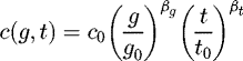
The second relationship (Eq. (2)) introduced by the authors is also a power-relation. This time, β represents the elasticity of unit costs in relation to grades; g0 and c0 are calibration parameters.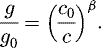 (2)
(2)
Different versions of this relationship can be found in the literature. While Schneider makes the simple assumption that β = 1 before looking at sensitivity, the MIT study introduces a more complex expression of β to take account of learning effects in addition to economies of scale. Finally, different versions of the relationship can be found depending on the value of β, either imposed or fitted. A number of them are gathered in Schneider and Sailor paper [6].
2.3 Step 3: cost-quantity model
Once the previous two relations are defined, step 3 derives the cost-quantity relationship from equations (1) and (2), according to equation (3).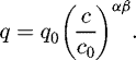 (3)
(3)
In this formula, the product denoted by αβ can be interpreted as the global elasticity of supply to unit costs of production. The LTCS curve is finally obtained by plotting the relationship of equation (3), once all parameters have been fitted or calibrated. Figure 3 shows the LTCS curves presented by Schneider for different versions of the previous framework1.
2.4 Limits of the elastic crustal abundance models
At this stage, several shortcomings can be raised against the framework proposed by Schneider, Matthews and Driscoll. First, the results are sensitive to calibration (Sect. 2.4.1). Second, only one intrinsic parameter of the resource, i.e. its grade, is used to determine both the geological availability (Eq. (1)) (Sect. 2.4.2) and the economic value of the resource (Eq. (2)) (Sect. 2.4.3).
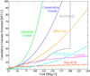 |
Fig. 3 Long-term cumulative supply curves for different versions of the elastic crustal abundance model [6]. |
2.4.1 Sensitivity to calibration (Eq. (3))
The final equation (Eq. (3)) for the LTCS curve requires a calibration point denoted by (q0, c0). Although Schneider investigates the sensitivity of αβ through different versions of his model (Fig. 3), the sensitivity to calibration is not covered. This paper conducts this sensitivity analysis according to the following methodology.
The cumulative resources (q0) and the corresponding cost limits (c0) were taken from various editions of the Red Book. To run the following sensitivity tests, the version of the elastic crustal abundance model that was used is Schneider's ‘optimistic crustal’ model (αβ = 3.32). Table 1 presents the different calibration points that were considered and Figure 4 shows the resulting sensitivity.
Figure 4 shows how the choice of the calibration points affects the LTCS curve.
Calibration points (c0,q0).
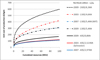 |
Fig. 4 Sensitivity of the elastic crustal abundance model in relation to calibration points. |
2.4.2 Limits to quantity-grade relationship (Eq. (1))
In the late 1970s, Deffeyes and Macgregor [9] reported imperfections in the bell-shape distribution of the grades. They noted that in the case of chromium, but also uranium, certain high grades can be overrepresented compared to the theoretical model, as shown in Figure 5.
Deffeyes explained this kind of bimodal distribution by particular forms of mineralization. These would be formed by a different sequence of independent phenomena compared to the sequence of the main distribution and result in a separate distribution. This point is important since it was shortly after Deffeyes’ publications that the main very high-grade deposits of Saskatchewan in Canada were discovered (Cigar Lake in 1981, McArthur River in 1988). The inclusion of these deposits in the diagram of Figure 2 invalidates the bell-shape model used in Schneider's and Matthews’ methods.
2.4.3 Limits to the cost-grade relationship (Eq. (2))
Apart from scale effects, considering the unit cost of production as only a function of grade can be opened to criticism. Today, some running uranium mines, which must have similar total production costs to be competitive in the current market, have substantially different grades [10]:
-
Cigar Lake, Canada (underground, 14.4% U, $23/lb U3O8 nominal operating cost);
-
South Inkai, Kazakhstan (in situ leaching, 0.01% U, $22/lb U3O8 nominal operating cost).
Conversely, some projects of similar grades may have quite different production costs [10]. In the following example, the production cost for in situ leaching is mainly operating cost, whereas for open pit, capital costs cannot be omitted:
-
Carley Bore, Australia (in situ leaching, 0.03% U, $20/lb U3O8 nominal operating cost);
-
Letlhakane, Botswana (open pit, 0.02% U, $58/lb U3O8 nominal operating cost).
As a consequence of the limits of the two previous relationships, the outputs of the model are not robust: as suggested in Figure 3, different values for the elasticity parameters αβ can change the output significantly and no acceptable conclusion on available resources can be found.
While grade is certainly an important factor in the cost of a resource, there are other parameters that govern cost and it may be desirable to model them. These include the size of ore bodies and the geochemical nature of deposits. Any change in these parameters can lead to specific mining techniques and therefore specific costs. When a deposit is located in a given country with specific legislation, taxes and royalties can also be taken into account through the cost.
Thus, if the cost function keeps a limited number of parameters, it can be more realistic to calibrate each deposit category or geological environment individually (one calibration for Canadian underground mines, one calibration for Australian ISL mines, etc.).
3 A statistical approach based on geological environments
To overcome the limits of previous models, this paper proposes a statistical approach that differs on three points from the elastic crustal abundance models:
-
geological availability and production costs are estimated by a bivariate model. The two variables are grade (mean grade of a deposit, denoted g) and tonnage (ore tonnage of a deposit, denoted t);
-
the scope of the model is split to several regional crustal abundance estimations. These regions are called geological environments2. A geological environment is defined by its own geographical boundaries, resource dispersion (average grade and size of ore bodies and their variance), and cost function;
-
a statistical approach is adopted. Variables g and t are treated as random variables and their probability density functions (pdfs) serve to build the corresponding relationship.
Section 3.1 briefly presents former geostatistical models, which have been applied to uranium endowment and share the same framework as the one developed in this article. Then Sections 3.2 to 3.4 describe the methodology step-by-step.
3.1 Former geostatistical models
Several bivariate or multi-variate statistical models for crustal abundance and associated costs can be found in the literature. Their objectives are the same as in Section 2 but rather than proceeding to the economic appraisal of cumulative quantities, statistical models proceed to the economic appraisal at a deposit level and then add up all the resources of deposits. The benefit of this approach is that models can be specific to each geological environment.
Among the models available in the literature, three have been applied to uranium endowment estimation. They were developed by Drew [11], Harris et al. [12–15] and Brinck [16–18]. None of them served to build a complete LTCS curve (rather they served to estimate the undiscovered resources at below a given cost, i.e. the price of U3O8 at the time of the studies), but some parts inspired the model developed in this paper. The general framework can be described in three parts which differ a little from the three steps described in Section 2:
-
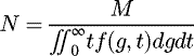
For a specific environment, the geological abundance q can be defined using a constant q0, the total metal endowment of the geological environment, and a probability density function f(g,t) (Eq. (4)):
 (4)
(4)
q0 is estimated from the mass of rock M in the geological environment and the mean grade of the crust (clarke) (q0 = M × clarke). It should be noticed that this q0 has no embedded consideration about economics nor technical recovery, unlike the calibration values used in Section 2.3.
q is derived from the statistics of g and t among the known deposits of a given geological environment. Since these statistics are biased (high-grade and high-tonnage deposits tend to be first discovered), a specific method is required to derive the unbiased function f(g,t). This method is based on economic filtering.
-
The second part consists in a cost model which is similar to that of elastic crustal abundance models, except costs are estimated at a deposit level and ore tonnage is taken into account. The resulting cost-grade-tonnage relationship is of the form described by equation (5), which can be also written as in equation (6) with x = ln(g), y = ln(t) and A a constant.
 (5)
(5)
 (6)
(6)
-
In part 3, Drew proposes to compute the cumulated metal resources available at below a given unit production cost C1 by using to intermediate calculations: the numerical computation of N, the total number of deposits in the environment (the total mass of rock M divided by the mean tonnage of all deposits), and m (C1), the mean metal content of deposits that are “cheaper than C1”. Equations (7) and (8) give the analytical expressions of N and m (C1) in terms of statistical expectations.
 (7)
(7)
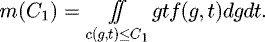 (8)
(8)
Finally, the LTCS curve is built by plotting the function C1 → N × m(C1 ).
In this paper, the numerical method used to derive the parameters of the unbiased function f(g,t) (part 1) is inspired from Drew, except for the cost limit used by the economic filter (see Sect. 3.3.2). The general form of the cost-grade-tonnage relationship (part 2, Eq. (5)) is also inspired from Drew and Harris, but its calibration is a different procedure (see Sect. 3.3.1). Lastly, the numerical procedure used to compute the cumulated resources available at a given cost (part 3) is specific to this paper (see Sect. 3.4).
Apart from Harris, Brinck and Drew's models, a more advanced approach has been proposed by the United States Geological Survey (USGS): “Quantitative Mineral Resources Assessments” [19,20]. Although this methodology is often referred to as “3-part resource assessment”, these parts are not exactly the same as the three parts of our general framework. Neither are the objectives: within a given geological environment (e.g. United States), tracts are delineated (e.g. a sandstone basin in New Mexico) and mapped data available on these tracts are analysed in order to find similarities with unexplored or less explored tracts. The output is not only an estimation of undiscovered resources but also the density and target location of undiscovered deposits. This localization dimension is missing in our approach since it is not in the scope of this research, without mentioning the difficulty to gather consistent and extensive mapped data for grade and tonnage over large areas such as geological environments.
3.2 Part 1: abundance model
3.2.1 Log-normal distribution of grade and tonnage
The purpose of part 1 is to characterize the density function f, i.e. the statistical distribution of grade and tonnage among the deposits of the geological environment being considered. It is common, although sometimes criticized, to assume that f follows a bivariate log-normal distribution [13]. (Since g and t follow log-normal distributions, x = ln(g) and y = ln(t) follow normal distributions.) This assumption is shared with Harris, Brinck and Drew's models. It leads to the mathematical form described by equation (9), provided that grade and tonnage are independent random variables3.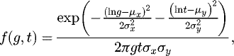 (9)where μx, σx2 and μy, σy2 are the means and variances of x and y respectively.
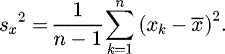
The most technical part of part 1 is to estimate those parameters from statistical data on known deposits. In descriptive statistics, mean and variance are computed according to equations (10) and (11).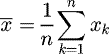 (10)
(10)
 (11)
(11)
If deposits were randomly sampled and n large enough, equations (10) and (11) would be the best estimators of μx and σx2 (μy and σy2 respectively) 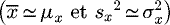 . Unfortunately, deposits are not randomly sampled. Rather, the richer (high grade, high tonnage) raise economic interest first.
3.2.2 Economic filter and procedure to estimate the parameters of the unbiased distribution
The procedure used in this paper is derived from Drew [11,14]. Harris and Drew propose similar procedures to correct for the sampling bias that affects known deposits [14]. Their idea is to model an economic filter. This filter is a function that truncates the density function of deposits, i.e. f. Thus, deposits are split between observable and non-observable deposits, based on a given cost limit and their economic value.
With this filter, empirical data correspond to observable deposits. Because of truncation, grade and tonnage of observable deposits do not follow a log-normal distribution anymore. Rather, they follow a truncated log-normal distribution. The truncation limits (glim and tlim) are related to a given cost limit Clim through a cost-grade-tonnage relationship which characterizes the economic filter.
Drew and Harris propose to use the same kind of relationship as in part 2 (Eqs. (5) and (6)):

When glim and tlim are known, the probability density functions (pdfs) of truncated log-normal distributions have explicit expressions that can be related to the non-truncated pdf [14]. Indeed through mathematical manipulations, Drew showed that the statistical expectations (mean value) for grade, tonnage and metal content (respectively denoted γg, γt, γm) on the truncated population could be expressed in terms of the unknowns μx, σx2 and μy, σy2. This is shown in equations (12) to (14). (12)
(12)
 (13)
(13)
 (14)
(14)
where: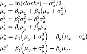 (15)
(15)
Since bias has been taken into account, γg, γt and γm are the theoretical value of the empirical estimators  (Eq. (10) applied to g, t, and m = g × t). If γg, γt and γm are replaced by these empirical values in equations (12) to (14), the system consists of 3 equations and 4 unknowns. It can be solved using the additional constraint of equation (15). The solution tuple (μx, μy, σx, σy) can be numerically found by using an optimization routine that minimizes the error Δ defined in equation (16).
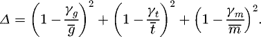 (16)
(16)
3.3 Part 2: cost-grade-tonnage relationship
3.3.1 Calibration of the cost-grade-tonnage relationship
The form of the cost-grade-tonnage relationship (Eq. (5)) is chosen by Harris and Drew to handle a linear form in the log-space (see Eq. (6)). This is necessary to achieve the integrations of part 1 (when the relationship is used as economic filter) and part 3 (when it is used for the economic assessment of all deposits).
To calibrate the function, Drew and Harris first compute the theoretical total cost Ctot(g,t) of a symbolic deposit as if it was a mining project. They use the discounted cash flow (DCF) method with costs from abacus. Then parameters βg, βt and constants are optimized so that the unit cost c(g,t) from the relationship of equation (11) best fits the unit cost (Ctot(g,t)/(g × t)) computed for the symbolic deposit.
This paper follows the same methodology except for the computation of Ctot. Rather than using abacus which are not publicly available for current mines, we propose to compute Ctot from recent mines or recent projects whose capital costs CC, development time DT, operating costs OP, lifetime LT, grade and tonnage are known. The corresponding formula is given by equation (17) where a is the discount rate.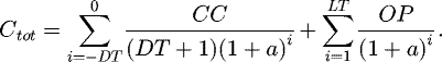 (17)
(17)
Once Ctot is computed for a set of deposits taken from the database (each having specific grade and tonnage), parameters βg and βt and constants were optimized so that the unit cost c(g,t) from the relationship of equation (6) best fits Ctot(g,t)/(g × t)4.
3.3.2 Use of the cost-grade-tonnage relationship
Once calibrated, the cost-grade-tonnage relationship is used in two different ways in part 1 and in part 3.
In part 1, it truncates the bivariate log-normal distribution in order to characterize observable deposits in today's economic conditions. To that end, unit cost is taken equal to a constant C, which can be fixed at the current long-term uranium price5. And from equation (6), minimal grade for any deposit of tonnage t to be observable is given by equation (18). Likewise, minimal tonnage for any deposit of tonnage g to be observable is given by equation (19). (18)
(18)
 (19)
(19)
In part 3, when the cost-grade-tonnage relationship is used, unit cost is the output (cf. Sect. 3.4).
3.4 Part 3: LTCS curve construction
Finally, when the distribution function f is known (Eq. (9)), any deposits from the geological environment can be simulated. In addition, once the cost-grade-tonnage relationship has been calibrated, the cost of each of these deposits can be estimated (Eq. (5)). Therefore, part 3 is the procedure that adds up the resources of deposits within a given cost range (Eqs. (7) and (8)).
The integral of equation (8) raises some difficulties as it cannot be solved analytically (essentially because the domain of integration is dependent upon g and t through c(g,t)). To compute a numerical approximation of the integral, Drew introduces the following variable substitution: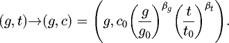
Using this substitution, the domain of integration of variable c is simplified (it is integrated from 0 to C1 as defined in Eq. (8)). But Drew does not mention the new domain of integration of variable g. In fact, before the substitution, g and t were independent random variables. But g is not, in any way, independent from  . Therefore, the mathematical expression used to compute the statistical expectation of equation (8) cannot stand for the computation of cumulated resources since the probability distribution of c is unknown.
For those reasons, this study developed an alternative numerical method to compute the cumulated metal resources available at below a given unit production cost C1. These quantities are estimated though a numerical approximation of the following integral derived from equation (4) with the relevant domain of integration: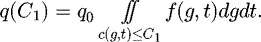 (20)
(20)
The numerical approximation consists in applying the rectangle method and introducing the following indicator function: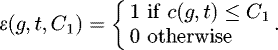 (21)
(21)
Hence, q can be approximated by the following sum: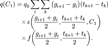 (22)
(22)
In equation (22), (gi) and (tk) are used as a mesh of the domain of integration. To ensure a precise approximation, the mesh and its refinement should be carefully defined. In this paper, we used a logarithmic mesh defined as follows:
The LTCS curve is finally obtained by plotting the function C1 → q(C1 ).
4 Preliminary results for the US endowment
The case of United States was chosen to validate the methodology developed in this paper. Several reasons have guided this choice. First, this country has a sustained history of uranium exploration and mining. The data required for this study are all available and generally quite extensive. Second, the United States has long experience in mineral appraisal assessment too (see the USGS “Quantitative Mineral Resources Assessments” [19,20]). Besides, Harris and Drew conducted similar economic appraisal of US resources. Although the results cannot be compared due to cost escalation since their studies (late 70 s, early 80 s), our model provides an up-date of uranium resource appraisals.
Since part 1 uses the calibrated cost relationship described in part 2, the database used for the calibration and the results of this calibration are presented first (Sects. 4.1.1 and 4.1.2). Then the database used for the deposit statistics is presented (Sect. 4.2.1). Finally, Section 4.2.2 and Section 4.3 gather the results of part 1 and part 3 applied to the US geological environment.
4.1 Calibration of the cost relationship
4.1.1 WISE Uranium cost database for US deposits
The WISE Uranium project gathers information on uranium mining activities around the world [10]. Among them are a list of mining companies, statistics of the mining industry and a list of known deposits with related recent issues. For 55 of those deposits, publicly available cost data are detailed so that for each of them capital costs CC, operating costs OP, lifetime LT, grade and resources are known. Fifteen of those deposits are located in United States. Twelve of them6 were used to estimate the parameters of equation (6) (βg, βt and the constant A). Table 2 gathers the total costs of these deposits. They were computed according to equation (17) based on the following assumptions:
-
tonnage t was computed as m/g where m includes all metal resources (indicated, inferred and measured, either reserves or resources) and g is the average grade of those resources;
-
life time was computed as the minimum of t/Kmill and m/Koverall where Kmill is ore processing capacity (in tonnes of ore per year) and Koverall is the overall production capacity (in tonnes of uranium per year);
-
discount rate is 10%;
-
development time is 3 years.
Total cost and ore tonnage of US deposits.
4.1.2 Results of part 2: cost function calibration
From the data of Table 2, a linear regression gives the following results: (23)
(23)
Unit production cost is obtained by dividing Ctot by m = g × t in equation (23) (where m is the metal content, g the mean grade and t the mean tonnage). Hence, we derive equation (24) where βg, βt and the constant A can be identified. (24)where βt = –0.499, βg = –1 and A = 11.61.
4.2 Calibration of the abundance model
4.2.1 UDEPO data for US deposits
IAEA provides a large database on uranium deposits called UDEPO [21]. This database gives a resource assessment on most known deposits in the world. It is based on available information and may not always be JORC or NI 43-1017 compliant. The database classifies the deposits based on a number of parameters including mean grade and corresponding metal content.
This paper uses the statistics of US deposits available in the UDEPO database (329 deposits8). Since ore tonnage is not an explicit parameter of the database it was approximated by m/g where m is the metal content and g is the mean grade. UDEPO has a lower cutoff on metal content: only deposits bigger than 300 tU are reported. Although there is a number of known deposits below this cutoff in the US, they would not influence the estimation of the log-normal parameters since only deposits above the economic filter are taken into account during the procedure of part 1. Table 3 presents the statistics of US deposits and Figure 6 shows the tonnage and the grade of both UDEPO deposits and WISE projects; the economic filter obtained from Section 4.1.2 (Eq. (24)) is also displayed for Clim = 125 $/kgU.
Statistics of known US deposits (UDEPO).
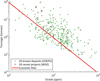 |
Fig. 6 Grade and tonnage of US known deposits and recent projects. |
4.2.2 Results of part 1: estimated log-normal parameters
Using the statistics of US deposits from UDEPO database, the optimization routine described in Section 3.2.2 is run, with the additional assumptions:
-
the mean grade of the crust within the geological environment, clarke, is taken equal to 3 ppm (eq. U3O8)9 = 2.54 × 10⁻⁶ kgU/kg of ore;
The resulting estimated parameters are:
-
μx = –15.26;
-
σx = 2.18;
-
μy = 13.63;
-
σy = 1.08.
The bias correction between these estimations and the original UDEPO statistics (Tab. 3) is noticeable. In particular, the mean grade is largely overestimated in UDEPO (μx = –15.26 <  = –6.76, see Tab. 4 for non-logarithmic comparisons) but standard deviation for grade is underestimated (σx = 2.18 > sx = 0.77). Regarding deposit size (y), the bias is also significant (we tend to discover bigger deposits first) but less markedly than for grade.
Those estimations of unbiased parameters can be compared with Harris and Drew's values (Tab. 4). Since the authors use different units for grade, all results are given for variables (g,t) in ppmU and tonnes. Conversion from (x,y) parameters to (g,t) parameters is given in equations (25) to (28) according to the definition of the log-normal distribution. (25)
(25)
 (26)
(26)
 (27)
(27)
 (28)
(28)
Table 4 shows significant differences on several points. First, the average ore tonnage of deposits,  , is much larger in this study than in Harris or Drew. Since this difference can already be seen in input statistics (biased statistics from known deposits), it can be explained by different definitions of deposits. Drew has certainly the most restrictive definition (probably taking only measured reserves to delineate deposits) while the UDEPO database used in this study has a less compelling definition (resources that do not comply with JORC/NI 43-101 are considered). These differences may not impact the construction of the LTCS curve if the cost-grade-tonnage relation is calibrated using the same resource definition. In this study, the deposits from Wise Uranium that are used for calibration include all resources (including inferred and indicated resources), as specified in Section 4.1.
In addition, there are also significant differences in the standard deviations for grade, Sg. This time, the difference cannot be noticed in input statistics:  (mean grade of known deposits) is similar in this study (1544 ppmU) and Harris (1560 ppmU) and so is sg (1299 ppmU in this study and 1076 ppmU in Harris’). This suggests that the definition of the deposit size can significantly influence the estimated standard deviation for grade during the bias correction procedure (Sect. 3.2.2).
Comparison of the biased empirical statistics with the estimated unbiased parameters for the log-normal distribution.
4.3 US LTSC curve
4.3.1 Results
Finally, the calibrated cost relationship obtained in Section 4.1.2 and the parameters of the bivariate log-normal distribution obtained in Section 4.2.2 can be used to build the US LTSC curve. The procedure is described in Section 3.4. In addition to the previous assumptions, the size of the US geological environment was assumed to be the total mass of rock, M, contained in the total US area to a depth of 2 km11. M = 4.24 × 10¹⁶ tonnes. The procedure also takes account of a 75% overall recovery rate12 (including extraction losses, ore sorting losses and processing losses).
The results are plotted in Figure 7.
Figure 7 shows the US LTCS curve obtained with the methodology developed in this paper (blue curve). It is compared with the US resource declaration available in the Red Book (2011 edition13 [24]) (red curves). It appears that the known resources (RAR) reported in the Red Book14 are more limited than the simulated US resource appraisal. This is expectable since past production and undiscovered resources are excluded from the Red Book RAR quantities. It is also noticeable that for costs falling below the Red Book limit of 130 $/kgU, the simulated endowment is more conservative than the expected total resources (known and undiscovered, RAR + PR + SR) reported in the Red Book.
 |
Fig. 7 US LTCS curve (logarithmic scale). |
4.3.2 Discussion
These results are preliminary outputs. Before further exploitation and analysis, some sensitivity tests are still necessary. Among the sensitivity parameters which require further investigations are:
-
the geological environment under study;
-
parameters related to this geological environment (maximum depth that define M, mean crust grade clarke);
-
parameters related to the cost-grade-tonnage relationship (βg, βt and A);
-
parameters specifically related to the economic filter (cost limit C used to define observable deposits).
5 Conclusion
For the purpose of analyzing the long-term availability of uranium resources, this paper develops a methodology to build long-term cumulative supply curves. After covering existing models and stressing their limits, a methodology based on geological environments is proposed. Its statistical approach provides a more detailed resource estimation and is more flexible regarding cost modelling. In particular, both grade and tonnage are considered in the economics of deposits and an economic filter is introduced to correct the observation bias that limits our knowledge to the richest deposits.
Preliminary results for the US endowment are presented. Although the model still requires some additional sensitivity tests, these results are promising. They showed a slightly more conservative endowment than the estimated undiscovered resources reported in the Red Book. The preliminary results validate the general methodology and could maybe allow for future comparison with alternative methodologies such as the USGS “3-part resource assessment”.
References
- A. Baschwitz, C. Loaec et al., Long-term prospective on the electronuclear fleet: from GEN II to GEN IV, in Global 2009: The nuclear fuel cycle: sustainable options & industrial perspectives , Paris, France (2009) [Google Scholar]
- S. Gabriel, A. Baschwitz et al., Building future nuclear power fleets: the available uranium resources constraint, Res. Pol. 38 , 458 (2013) [CrossRef] [Google Scholar]
- J.E. Tilton, B.J. Skinner, In The meaning of resources, edited by D.J. McLaren, B.J. Skinner, Resources and world development (John Wiley & Sons, New York, 1987) p. 13 [Google Scholar]
- J.E. Tilton, A. Yaksic, Using the cumulative availability curve to assess the threat of mineral depletion: the case of lithium, Res. Pol. 34 , 185 (2009) [Google Scholar]
- OECD NEA, IAEA, Uranium 2014: resources, production and demand (OECD Nuclear Energy Agency, Paris, France, 2014), p. 508 [Google Scholar]
- E.A. Schneider, W.C. Sailor, Long-term uranium supply estimates, Nucl. Tech. 162 , 379 (2008) [CrossRef] [Google Scholar]
- I.A. Matthews, M.J. Driscoll, A probabilistic projection of long-term uranium resource costs (Massachusetts Institute of Technology, Cambridge, Massachusetts, 2010), p. 141 [Google Scholar]
- Massachusetts Institute of Technology, The future of nuclear fuel cycle an interdisciplinary MIT study (Massachusetts Institute of Technology, Cambridge, Massachusetts, 2011), p. 258 [Google Scholar]
- K. Deffeyes, I. Macgregor, Uranium distribution in mined deposits and in the earth's crust (Princeton University, Princeton, New Jersey, 1979), p. 509 [Google Scholar]
- World Information Service on Energy, WISE Uranium Project (website), WISE Uranium, http://www.wise-uranium.org/index.html (accessed: 03/2015) [Google Scholar]
- M.W. Drew, US uranium deposits: a geostatistical model, Res. Pol. 3 , 60 (1977) [CrossRef] [Google Scholar]
- M.L. Chavez-Martinez, A potential supply system for uranium based upon a crustal abundance model (University of Arizona, Tucson, Arizona, 1982), p. 491 [Google Scholar]
- D.P. Harris, Quantitative methods for the appraisal of mineral resources (University of Arizona, Tucson, Arizona, 1977), p. 862 [Google Scholar]
- D.P. Harris, Mineral resources appraisal: mineral endowment, resources, and potential supply: concepts, methods and cases (Oxford University Press, Oxford, UK, 1984) [Google Scholar]
- D.P. Harris, In Geostatistical crustal abundance resource models, edited by C.F. Chung, A.G. Fabbri, R. Sinding-Larsen, Quantitative analysis of mineral and energy resources (Springer, Netherlands, 1988) p. 459 [CrossRef] [Google Scholar]
- J.W. Brinck, MIMIC - The prediction of mineral resources and long-term price trends in the non-ferrous metal mining industry is no longer utopian, Eurospectra 10 , 46 (1971) [Google Scholar]
- J.W. Brinck, Calcul des ressources mondiales d’uranium, Bull. Communaute Eur. Energie At. 6 , 109 (1967) [Google Scholar]
- H.I. de Wolde, J.W. Brinck, The estimation of mineral resources by the computer program ‘IRIS’ (Commission of the European Communities, Luxembourg, 1971) [Google Scholar]
- D.A. Singer, Short course introduction to quantitative mineral resource assessments (US Geological Survey, Menlo Park, California, 2007) [Google Scholar]
- D.A. Singer, W.D. Menzie, Quantitative mineral resource assessments — An integrated approach (Oxford University Press, New York, 2010), p. 219 [Google Scholar]
- IAEA, World Distribution of Uranium Deposits (UDEPO) (website), https://infcis.iaea.org (extensive copy of the database accessed: 11/2013) [Google Scholar]
- K. Hans Wedepohl, The composition of the continental crust, Geochim. Cosmochim. Acta 59 , 1217 (1995) [Google Scholar]
- UX Consulting, “UxC” (website), http://www.uxc.com (accessed: 03/2015) [Google Scholar]
- OECD NEA, IAEA, Uranium 2011: resources, production and demand (OECD Nuclear Energy Agency, Paris, France, 2012), p. 489 [CrossRef] [Google Scholar]
To be more correct, FCCCG(2) and DANESS models differ from the elastic crustal abundance model. These specific characteristics are not covered by this paper.
This terminology was first used in Drew [11]. It is convenient because the model produces an assessment of geological resources rather than reserves within the environment. Yet, the meaning of “geological” can be confusing. The boundaries do not aim to circle a single geological structure but rather groups of structures that share a maximum of common properties (types, size, grade of known deposits and also economic, political conditions) compared with other environments (e.g. US groups of deposits vs. Canada, Australia, Africa or Kazakhstan).
The question of the independence between grade and tonnage in mineral deposits is in constant discussion. Beside, in his research [14], Harris comes to the conclusion that in the case of biased observations, if any correlation exists, it could very well be mitigated, amplified or even totally concealed by the bias filter. In this paper, assumption is made that g and t are independent.
In their studies, Drew and Harris considered short-term prices (8 $/lbU3O8 in 1977 [11] and 50 $/lbU3O8 in 1988 [15]). Although no long-term index existed at that time, this choice is open to criticism, especially when spot prices fluctuated as they did in the late 1970s and more recently. Long-term price index was preferred in this study as it is more stable. The highest Red Book cost limit (260 $/kgU) could have been considered as well but since this price has never been reached over long periods, it is expected that this cost category only contains sparse data.
Two have incomplete data and Roca Honda mine seems to have abnormal data, perhaps because milling costs are omitted (milling occurs at White Mesa mill).
JORC and NI 41-101 are two national (Australian and Canadian respectively) sets of rules and guidelines for estimating and reporting mineral resources.
Three hundred and forty-two in total but 13 deposits were discarded. Three of them have incomplete data. Seven of them correspond to regional resource assessments (e.g. Northern Great Plains, Phosphoria Formation, Central Florida). Three of them are high-tonnage and very low-grade deposits where uranium is a by-product (Bingham Canyon, Yerington, Twin Butte).
March 2015.
A maximum depth of 2 km was preferred to Drew's value (1 km [11]) as some uranium mines are known at those depths.
This choice was guided by the Red Book [5] reference values (70 to 75% for underground and ISL methods which are the most common in the United States, and 75% when no method is specified).
In the 2014 edition, there is no declaration of US Prognosticated and Speculative resources (PR & SR). The 2011 edition was preferred for comparison purposes.
The US does not report inferred resources (IR).
Cite this article as: Antoine Monnet, Sophie Gabriel, Jacques Percebois, Statistical model of global uranium resources and long-term availability, EPJ Nuclear Sci. Technol. 2, 17 (2016)
All Tables
Comparison of the biased empirical statistics with the estimated unbiased parameters for the log-normal distribution.
All Figures
 |
Fig. 1 Long-term supply curve built from the 2014 Red Book data [5]. |
| In the text | |
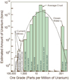 |
Fig. 2 Empirical bell-shape relationship between cumulated uranium resources and ore grades [9]. |
| In the text | |
|
Fig. 3 Long-term cumulative supply curves for different versions of the elastic crustal abundance model [6]. |
| In the text | |
|
Fig. 4 Sensitivity of the elastic crustal abundance model in relation to calibration points. |
| In the text | |
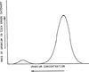 |
Fig. 5 Bimodal relationship between cumulated uranium resources and ore grades [9]. |
| In the text | |
|
Fig. 6 Grade and tonnage of US known deposits and recent projects. |
| In the text | |
|
Fig. 7 US LTCS curve (logarithmic scale). |
| In the text | |
Current usage metrics show cumulative count of Article Views (full-text article views including HTML views, PDF and ePub downloads, according to the available data) and Abstracts Views on Vision4Press platform.
Data correspond to usage on the plateform after 2015. The current usage metrics is available 48-96 hours after online publication and is updated daily on week days.
Initial download of the metrics may take a while.