© E. Vandermeersch et al., Published by EDP Sciences, 2021

1 Introduction

Massimo Salvatores kept a constant and dedicated interest in perturbation theory aimed at the quantification of sensitivities and uncertainties, contributing many now legacy methods. Recently, he played an inspirational role in two specific examples. The first one was about surpassing the traditional multigroup description to reach a kind of continuous energy treatment of nuclear data sensitivities and associated uncertainties [1,2]; the second one was about discrete, multipoint descriptions in the frame of coupled core theories and the quantification of the sensitivity of coupling coefficients to nuclear data [3]. The scope of this tribute paper is to review briefly some recent achievements in these thematic lines. Section 2 is devoted to the determination of continuous energy sensitivities to a discrete set of nuclear parameters and Section 3 to a reduced-cost, deterministic calculation of the sensitivity of multipoint source distributions to nuclear data.

2 Sensitivities to nuclear parameters

Deployments of new models in nuclear physics confirm the need for more consistency in the integral experiment assimilation process: currently, assimilation is usually achieved onto nuclear data (mainly cross sections alone), instead of the nuclear parameters at the origin of these data. Such a feedback may lead to non-physical nuclear data. This lack of consistency could be surpassed by ensuring that all the nuclear data used during a simulation come from the same parameters and theoretical models, before applying the assimilation process to the nuclear parameters themselves. To carry out this process, we have implemented a soft coupling between the nuclear data evaluation code CONRAD [4,5] and the stochastic transport code TRIPOLI-4® [6].

2.1 Nuclear data evaluation

Depending on the incident neutron energy, nuclear data are obtained from different models and parameters: in the resolved resonance range, with the R-matrix formalism [7], the various resonances widths Γ and positions E_λ (usually obtained experimentally) are sufficient to obtain cross sections and angular distributions values. At higher energy (in the so-called continuum), resonances cannot be distinguished experimentally, and the nucleus is described (partly) by the optical model [8]. To compute nuclear data, this model uses a parametrized potential [8] to fit experimental data. Nuclear parameters, in this model, describe, for example, geometrical aspects (radius, diffuseness), potential depth (V_HF). At these energies, more models, not detailed here, are also required to describe more precisely neutron-nucleus interactions, such as fission.

The C++ CONRAD [4,5] code allows us to produce consistent nuclear data, and to compute their sensitivities to nuclear parameters. It is developed at LEPh (CEA-Cadarache) to perform nuclear data evaluation, analysis and integral experiment assimilation. This nuclear evaluation code can produce nuclear data for all the energy range used in neutronics: from a set of nuclear parameters, the code is able to produce cross sections, angular distributions and energy distributions for radiative capture, fission, elastic and inelastic scattering reactions. For the resolved resonance range (R-matrix), CONRAD possesses its own solver. For the continuum, total cross sections are computed with either its own solver or the code ECIS. For partial reactions, CONRAD calls the nuclear data code TALYS [9], to compute cross sections, angular and energetic distributions (for the inelastic continuum) at each point of the energy grid asked, or automatically determined.

Regarding fission, CONRAD currently evaluates only prompt neutron multiplicity, with a simple model based on linear energy of the incident neutron dependence. All those data are gathered into one GND evaluation file [10] and post-processed with the codes FUDGE, NJOY and TRIPOLI-4® into ENDF [11] and XDR (TRIPOLI-4®) files.

This first step of the coupling ensures that all nuclear data are produced with the same models and parameters, and allows continuous energy simulations with perturbed nuclear parameters, without restriction of energy domain or theoretical model. The second step of the coupling consists of using a development version of TRIPOLI [12], where the Iterated Fission Probability method (IFP) [13] is used to compute reactivity sensitivities to nuclear data, and has been extended with the CONRAD code to compute reactivity sensitivities to nuclear parameters [14].

2.2 Sensitivity computation

The steady-state neutron flux in a nuclear reactor is described by the deterministic Boltzmann equation:$$\left(\frac{F}{k}-A\right)\Phi =0$$(1) (with usual notations, $\Phi \left({\displaystyle \overrightarrow{r}},E,{\displaystyle \overrightarrow{\Omega }}\right)$ is the neutron flux, F is the neutron production operator, A groups all other operators in the Boltzmann equation, k is the multiplication factor). The boundary condition retained is no incoming flux on the (assumed convex) surface S defining the boundary of the system: $\Phi \left({\displaystyle \overrightarrow{r}},E,{\displaystyle \overrightarrow{\Omega }}\right)=0$ for ${\displaystyle \overrightarrow{r}}$ on S and, ${\displaystyle \overrightarrow{\Omega }}{\displaystyle \overrightarrow{n}}{\displaystyle \overrightarrow{n}}$ being the outward-pointing unit vector normal to S. This is an eigenvalue problem, with a unique dominant eigenpair (k, Φ); the problem being homogeneous, only the shape of the flux is determined, its level is arbitrary (this scale factor can be used to normalize the flux, e.g. to a prescribed reactor power). We also use the following notations for integrals and inner products of functions:$$⟨\varphi ⟩=\int \varphi \left({\displaystyle \overrightarrow{r}},E,{\displaystyle \overrightarrow{\Omega }}\right)d^{3}rdE{d}^2\Omega$$ $$⟨\varphi ,\psi ⟩=\int \varphi \left({\displaystyle \overrightarrow{r}},E,{\displaystyle \overrightarrow{\Omega }}\right)\psi \left({\displaystyle \overrightarrow{r}},E,{\displaystyle \overrightarrow{\Omega }}\right)d^{3}rdE{d}^2\Omega$$(2)

As usually defined in linear algebra, the adjoint of operator Q is operator Q ⁺ such as:$$\forall \left(\varphi ,\psi \right):\text{▓}⟨\varphi ,Q\psi ⟩=⟨Q^{+}\varphi ,\psi ⟩$$(3)

In a nuclear reactor, the adjoint flux is defined as a solution of the eigenvalue equation involving the adjoint operators of the standard equation:$$\left(\frac{F^{+}}{k}-A^{+}\right){\Phi }^{+}=0$$(4)

The boundary condition, chosen here to ensure the adjoint of the transport operator $\left({\displaystyle \overrightarrow{\Omega }}\cdot {\displaystyle \overrightarrow{\nabla }}\right)$ to be $\left(-{\displaystyle \overrightarrow{\Omega }}\cdot {\displaystyle \overrightarrow{\nabla }}\right)$, is no outcoming adjoint flux on S: ${\Phi }^{+}\left({\displaystyle \overrightarrow{r}},E,{\displaystyle \overrightarrow{\Omega }}\right)=0$ for ${\displaystyle \overrightarrow{r}}$ on S and ${\displaystyle \overrightarrow{\Omega }}\cdot {\displaystyle \overrightarrow{n}}>0$. Equivalently to the multiplication factor k, the reactivity ρ is used very often and is defined as:$$\rho =\frac{k-1}{k}$$(5)

The sensitivity of the reactivity to a nuclear parameter Γ can be computed by summing the contribution to the sensitivity through each nuclear data (cross-section σ, angular distribution (AD) or energy distribution (ED)), as shown in equation (6):$$S_{\Gamma }^{\rho }=S_{\Gamma }^{\rho /\sigma }+S_{\Gamma }^{\rho /AD}+S_{\Gamma }^{\rho /ED}$$(6)

Angular and energy distributions are described here with the forwarding function f_r (ϵ → ϵ^′), which is the probability of a particle in the phase state ϵ to be scattered or emitted at the state ϵ^′ after the reaction r.

2.2.1 Finite difference approach

The naive way to compute reactivity sensitivities to nuclear parameters is to apply a finite difference approach. One nuclear parameter is perturbed to obtain two nuclear data evaluations, and the reactivity difference obtained after transport simulation is used to compute the sensitivity, as detailed in equation (7). The contributions of all nuclear data are calculated implicitly in the sensitivities. Unfortunately, this method implies two Monte Carlo computations, representing two symmetrical perturbations, for each required sensitivity. It also requires a very good convergence, especially if the parameter impact is small and thus is computationally very expensive.$$S_q^{\rho }=\frac{\partial \rho }{\partial q}\frac{q}{\rho }\approx \frac{{\rho }_{\text{reference}}-{\rho }_{\text{pertubed}}}{q_{\text{reference}}-q_{\text{perturbed}}}\frac{q_{\text{reference}}}{{\rho }_{\text{reference}}}$$(7)

2.2.2 Iterated fission probability

A more elegant method involves perturbation theory [15]. Until the last decade, adjoint-based methods for sensitivity computation were restricted to deterministic codes. Since Nauchi's [13] demonstration, such methods have been implemented in multiple ways in reference Monte Carlo codes. B. Kiedrowski has made an exhaustive review of the different methods in continuous energy codes [16]. We will focus here on the IFP method implemented in a development version of TRIPOLI-4®.

Perturbation theory allows expressing the sensitivity of reactivity ρ to the parameter q (nuclear data or nuclear parameter):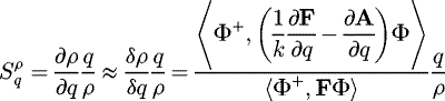$$S_q^{\rho }=\frac{\partial \rho }{\partial q}\frac{q}{\rho }\approx \frac{\delta \rho }{\delta q}\frac{q}{\rho }=\frac{{\Phi }^{+},\left(\frac{1}{\text{k}}\frac{\partial F}{\partial q}-\frac{\partial A}{\partial q}\right)\Phi }{{\Phi }^{+},F\Phi }\frac{q}{\rho }$$(8)

In order to estimate the adjoint flux of a system in a continuous transport code, at phase space point $ϵ=\left({\displaystyle \overrightarrow{r}},E,{\displaystyle \overrightarrow{\Omega }}\right)$, Nauchi [13] has demonstrated that one can use the importance I of a neutron at the same point. I (ϵ) is the average number of fissions produced by the neutron studied and its descendents: the more fissions it fathers, the more important is the neutron to the system. To compute the number of fissions produced, one usually propagates the studied neutron for L generations, and computes the normalization factor k_g of each generation g (called k_step in some continuous transport code). k_g is the number of neutrons produced at generation g. It has for name “normalization factor” as it serves, in Monte Carlo code, to normalize neutrons weights during the simulation.

As shown in equation (9), the importance is estimated with the normalization factor k_g. Such an estimator is already available in most Monte Carlo codes. Thus, one can easily estimate the adjoint flux of a system, with a large amount of small Monte Carlo simulations: for a simple critical system, convergence is reached after ten generations [12]. To avoid divergence, the importance should be normalized by the k_g after an infinite number of generations. Here, such a normalization is optional, as we compute a ratio of adjoint-weighted values.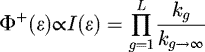$${\Phi }^{+}\left(ϵ\right)\propto I\left(ϵ\right)={\displaystyle {\displaystyle \prod }_{g=1}^L}\frac{k_g}{k_{g\to \infty }}$$(9)

Aufiero [17] has first used the IFP method for resonance parameter sensitivity calculation in continuous energy simulation. However, his method only allows sensitivity computation through nuclear parameter perturbations and is restricted to the resolved resonance model because of NJOY usage. The coupling presented here should allow computing sensitivities to any type of nuclear parameters, without model restriction.

2.2.3 Nuclear data contribution to nuclear parameters sensitivities

In order to obtain each of the contributions detailed in equation (6), we decided to decompose the sensitivity as shown in equation (10). Thus, the cross section contribution to the reactivity sensitivity to nuclear parameter Γ is expressed by: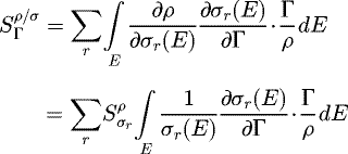$$S_{\Gamma }^{\rho /\sigma }={\displaystyle {\displaystyle \sum }_r}{\displaystyle \underset{E}{{\displaystyle \int }}}\frac{\partial \rho }{\partial {\sigma }_r\left(E\right)}\frac{\partial {\sigma }_r\left(E\right)}{\partial \Gamma }\cdot \frac{\Gamma }{\rho }dE={\displaystyle {\displaystyle \sum }_r}{S}_{{\sigma }_r}^{\rho }{\displaystyle \underset{E}{{\displaystyle \int }}}\frac{1}{{\sigma }_r\left(E\right)}\frac{\partial {\sigma }_r\left(E\right)}{\partial \Gamma }\cdot \frac{\Gamma }{\rho }dE$$(10)

Energy integration is done by summing derivative estimators over all the collisions simulated. Reactivity sensitivities to nuclear data are computed with the help of the theory of perturbations, and weighted by nuclear data sensitivities to nuclear parameters from CONRAD.

Reactivity sensitivities to the cross section of the reaction r can be estimated by: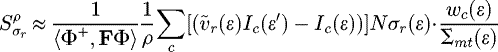$$S_{{\sigma }_r}^{\rho }\approx \frac{1}{{\Phi }^{+},\mathbf{F}\Phi }\frac{1}{\rho }{\displaystyle {\displaystyle \sum }_c}\left[\left({{\displaystyle \tilde{v}}}_r\left(ϵ\right)I_c\left({ϵ}^{\prime }\right)-I_c\left(ϵ\right)\right)\right]N{\sigma }_r\left(ϵ\right)\cdot \frac{w_c\left(ϵ\right)}{{\Sigma }_{mt}\left(ϵ\right)}$$(11)where ${{\displaystyle \tilde{V}}}_r$ is the number of neutrons emitted by reaction r, I_c the importance of the neutron at phase space point ϵ and for collision c, w the simulation neutron weight, N the nucleus concentration section of the collision medium, and Σ_mt the macroscopic cross section of the collision medium. For each collision, and each reaction, one should estimate the absorption and the emission contributions. The absorption contribution needs the importance of the incident neutron I (ϵ). The emission contribution also needs the importance of the outgoing neutron I_c (ϵ^′). For multiple emissions reaction, one can sample the importance of one of the emitted neutron, and use the multiplicity of the reaction. The fission production term ⟨Φ⁺, FΦ⟩ is expressed by: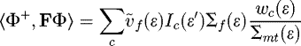$${\Phi }^{+},\mathbf{\text{F}}\Phi ={\displaystyle {\displaystyle \sum }_c}{{\displaystyle \tilde{v}}}_f\left(ϵ\right)I_c\left({ϵ}^{\prime }\right){\Sigma }_f\left(ϵ\right)\frac{w_c\left(ϵ\right)}{{\Sigma }_{mt}\left(ϵ\right)}$$(12)

The expression ⟨Φ⁺, FΦ⟩ will be kept in the Monte Carlo estimator to lighten the equations. The flux Φ is computed with the classical collision flux estimator: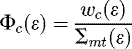$${\Phi }_c\left(ϵ\right)=\frac{w_c\left(ϵ\right)}{{\Sigma }_{mt}\left(ϵ\right)}$$(13)

Combining this with the decomposition from equation (8), we obtain equation (11):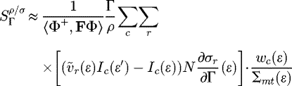$$S_{\Gamma }^{\rho /\sigma }\approx \frac{1}{{\Phi }^{+},\mathbf{\text{F}}⟩}\frac{\Gamma }{\rho }{\displaystyle {\displaystyle \sum }_c}{\displaystyle {\displaystyle \sum }_r}\left[\left({{\displaystyle \tilde{v}}}_r\left(ϵ\right)I_c\left({ϵ}^{\prime }\right)-I_c\left(ϵ\right)\right)N\frac{\partial {\sigma }_r}{\partial \Gamma }\left(ϵ\right)\right]\cdot \frac{w_c\left(ϵ\right)}{{\Sigma }_{mt}\left(ϵ\right)}$$(14)

The angular forwarding function f_r and the neutron spectrum χ do not appear in this sensitivity expression as there are implicitly sampled during the Monte Carlo simulation. Indeed, sensitivities are computed from pre-simulated collision histories.

Where Aufiero's method [17] is restricted to compute sensitivities through cross sections, CONRAD allows us to go further and compute other nuclear data contributions. Indeed, the same process can be applied to compute the sensitivity contribution through the angular forwarding function f_r: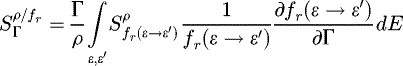$$S_{\Gamma }^{\rho /f_r}=\frac{\Gamma }{\rho }{\displaystyle \underset{ϵ,{ϵ}^{\prime }}{\int }}{S}_{f_r\left(ϵ\to {ϵ}^{\prime }\right)}^{\rho }\frac{1}{f_r\left(ϵ\to {ϵ}^{\prime }\right)}\frac{\partial f_r\left(ϵ\to {ϵ}^{\prime }\right)}{\partial \Gamma }dE$$(15)f_r is usually expressed with Legendre polynomials P_l and their associated coefficients a_l: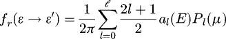$$f_r\left(ϵ\to {ϵ}^{\prime }\right)=\frac{1}{2\pi }{\displaystyle {\displaystyle \sum }_{l=0}^{\ell }}\frac{2l+1}{2}{a}_l\left(E\right)P_l\left(\mu \right)$$(16)

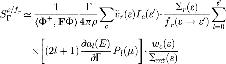
One can estimate reactivity sensitivity to f_r by: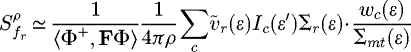$$S_{f_r}^{\rho }\simeq \frac{1}{{\Phi }^{+},\mathbf{\text{F}}\Phi }\frac{1}{4\pi \rho }{\displaystyle {\displaystyle \sum }_c}{{\displaystyle \tilde{v}}}_r\left(ϵ\right)I_c\left({ϵ}^{\prime }\right){\Sigma }_r\left(ϵ\right)\cdot \frac{w_c\left(ϵ\right)}{{\Sigma }_{mt}\left(ϵ\right)}$$(17)

And the reactivity sensitivity to the nuclear parameter $S_{\Gamma }^{\rho /f_r}$:$$S_{\Gamma }^{\rho /f_r}\simeq \frac{1}{{\Phi }^{+},\mathbf{\text{F}}⟩}\frac{\Gamma }{4\pi \rho }{\displaystyle {\displaystyle \sum }_c}{{\displaystyle \tilde{v}}}_r\left(ϵ\right)I_c\left({ϵ}^{\prime }\right)\cdot \frac{{\Sigma }_r\left(ϵ\right)}{f_r\left(ϵ\to {ϵ}^{\prime }\right)}{\displaystyle {\displaystyle \sum }_{l=0}^{\ell }}\left[\left(2l+1\right)\frac{\partial a_l\left(E\right)}{\partial \Gamma }{P}_l\left(\mu \right)\right]\cdot \frac{w_c\left(ϵ\right)}{{\Sigma }_{mt}\left(ϵ\right)}$$(18)

One can observe that the sensitivity contribution through the angular forwarding function does not depend on the incoming neutron importance. By expanding equation (8), the angular forwarding function and the neutron spectrum only appear on the production side of the neutron balance: sensitivity contributions will then only depend on the outgoing neutrons importances.

Even if a different set of nuclear parameters is involved, the method allows computing sensitivities of reactivity to prompt neutron spectrum parameters. The sensitivity obtained is detailed in equation (19), with χ_p the prompt neutron spectrum and β the delayed neutron fraction. This last contribution is set to zero here, as CONRAD is currently not able to produce such a spectrum.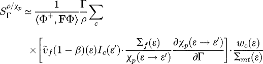$$S_{\Gamma }^{\rho /{\chi }_p}\simeq \frac{1}{⟨{\Phi }^{+},\mathbf{\text{F}}\Phi ⟩}\frac{\Gamma }{\rho }{\displaystyle {\displaystyle \sum }_c}\left[{{\displaystyle \tilde{v}}}_f\left(1-\beta \right)\left(ϵ\right)I_c\left({ϵ}^{\prime }\right)\cdot \frac{{\Sigma }_f\left(ϵ\right)}{{\chi }_p\left(ϵ\to {ϵ}^{\prime }\right)}\frac{\partial {\chi }_p\left(ϵ\to {ϵ}^{\prime }\right)}{\partial \Gamma }\right]\cdot \frac{w_c\left(ϵ\right)}{{\Sigma }_{mt}\left(ϵ\right)}$$(19)

The IFP method implemented in this development version of TRIPOLI-4® runs a first standard Monte Carlo simulation, and stores all collisions. For each collision, the neutron importance variation is computed by small Monte Carlo simulations. The sensitivities are computed from the data previously stored with a post-processing code called JIMMY. CONRAD is coupled to JIMMY in order to compute sensitivities to nuclear parameters.

2.3 Results

The method was tested on two simple plutonium-based benchmarks from the ICSBEP suite [18]: the first one, called the Plutonium Solution Thermal benchmark (PST001) consists of a spherical solution of multiple plutonium nitrates (radius of 14.5 cm), in a thin clad of steel (∼0.1cm thick), reflected by water. The second one, called the Plutonium Metal Fast benchmark (PMF001) is a simple bare sphere (6.4 cm radius) of plutonium-gallium alloy. Plutonium-239 parameters used come from the JEFF3.2 evaluation [19] and from future evaluations currently in production at CEA. Isotopic compositions are detailed in Table 1:

The two methods are compared with the estimator Δ/σ, defined, for two scores A and B and their uncertainties σ_A and σ_B, by: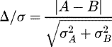$$\Delta /\sigma =\frac{\left|A-B\right|}{\sqrt{{\sigma }_A^2+{\sigma }_B^2}}$$(20)

As we use Monte Carlo simulation, results dispersion follows a Gaussian distribution. If Δ/σ < 3, for 99.7% of cases, the difference in the two methods comes from statistical fluctuations.

2.3.1 Sensitivities to resonance parameters

The PST001 offers a thermal neutron spectrum, suggesting high sensitivities to first the plutonium-239 resonances. The second advantage of plutonium-239 is its elastic isotropy at low energies, meaning that the reactivity sensitivities to resonance parameters only depend on cross section contribution. The results presented in Table 2 detail PST001 reactivity sensitivities to the first plutonium-239 positive-energy resonance: the resonance peak energy E₁, its neutron, gamma and fission widths Γ_N1, Γ_γ1, and Γ_F1. We compared the results obtained from finite difference method (by reconstruction of the perturbed nuclear data), to the one obtained from the coupling between the IFP method and CONRAD. Finite difference simulations have been completed with four million batches, and two thousand sources per batch.

The similarity between the results shows the efficiency of the IFP method in the Resolved Resonance domain: indeed, only one IFP computation is necessary to compute sensitivities to all nuclear parameters of all the isotopes needed, when the finite difference method needs two nuclear data evaluations and Monte Carlo simulations for each parameter.

Light nuclei are usually anisotropic in the R-matrix energy range. Thus, for these nuclei, sensitivities are dependent on angular distribution. We compared, as presented in Table 3, IFP and finite difference method with PST001 sensitivities to parameters of oxygen-16 second positive-energy resonance. These results show that the IFP method is able to manage sensitivities from different nuclear data contributions. For this benchmark, one sensitivity finite difference computation takes approximately 800 cpu.h (two simulations for a symmetric perturbation), compared to approximately 10000 cpu.h for the IFP method. One should remember that IFP method gives all the desired sensitivities in one calculation, unlike finite difference.

2.3.2 Sensitivities to optical model parameters

As anisotropy of heavy nuclei usually appears at fast neutron energies, it becomes necessary to work on higher energy to address the efficiency of the method for angular distribution contribution with heavy nuclei. At these energies, a new theoretical model has to be used (the optical model), implying different nuclear parameters. In this energy domain, CONRAD uses the TALYS code [9] to obtain nuclear data. We tested the method on the PMF001 benchmark, on the optical model nuclear radius r for plutonium-239, its diffuseness a and the depth of the Hartree-Fock mean-field potential well V_HF. It should be noticed that the plutonium nuclear data used here do not possess inelastic reactions to restrict the sensitivity contributions to cross section and angular distribution. Finite difference simulations have been completed with one million batches, three thousand sources per batch.

Results presented in Table 4 show again that the IFP method is able to manage sensitivities from multiple nuclear data contributions. Differences between the IFP method and the finite-difference method mostly come from elastic angular distribution contribution convergence, which accounts for 6 to 10% of all contribution in the results presented in Table 4. Because of the small number of collisions happening during a neutron life, computations are faster for this benchmark: 96 cpu.h for a finite difference computation, and 300 cpu.h for the IFP method.

2.3.3 Sensitivities to prompt neutron spectrum parameters

The method is valid for other kinds of nuclear data, as presented in Table 5. We managed to obtain sensitivity to prompt neutron spectrum parameters with the IFP method, with a reasonable correspondence to finite difference method sensitivities. Such results open the way for computation of sensitivities to delayed neutron parameters, unfortunately not available in the current CONRAD version.

3 Sensitivities of multipoint sources

Computation of the sensitivity of the coupling coefficients of a multipoint model of a reactor to nuclear data was achieved recently for a Monte Carlo modeling of the system [3]. In a deterministic model, making use of the Generalized Perturbation Theory (GPT) [15], this would require as many generalized importance calculations as there are coupling coefficients (i.e. n² for a system partitioned into n regions). Similarly, the GPT deterministic calculation of the sensitivity of the state eigenvector of a multipoint model to nuclear data requires as many generalized importance calculations as there are regions. We propose here a method to compute the sensitivity of this state eigenvector to nuclear data requiring only much simpler partial importance calculations. It was developed [20,21] as an original contribution. Although we could not find any reference to it, it is not excluded however, due to its simple algebraic structure, that similar ones might have been developed in the past.

3.1 Multipoint core model and coupling coefficients

The system under study obeys the deterministic Boltzmann equation (1). We will refer to this description as the “continuous” description of the system. The fissile volume of the system is partitioned into n separate volumes V₁, V₂, … , V_n and we want to assess the sensitivity of the discrete neutron production map over these volumes to nuclear data (cross-sections).

If δ_i is the characteristic function of volume V_i (i.e. δ_i (M) = 1 if point M is in volume V_i, δ_i (M) = 0 otherwise), the ratio of the neutron production in volume V_i to the global neutron production is: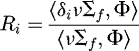$$R_i=\frac{⟨{\delta }_i\nu {\Sigma }_f,\Phi ⟩}{⟨\nu {\Sigma }_f,\Phi ⟩}$$(21)

The first-order variation of R_i is obtained using the classical Generalized Perturbation Theory (GPT, see e.g. [15]) as: 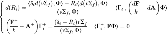$$\{\begin{array}{c}\hfill d\left(R_i\right)=\frac{⟨{\delta }_{i}d\left(\nu {\Sigma }_f\right),\Phi ⟩-R_i⟨d\left(\nu {\Sigma }_f\right),\Phi ⟩}{⟨\nu {\Sigma }_f,\Phi ⟩}-⟨{\Gamma }_i^{+},\left(\frac{dF}{k}-dA\right)\Phi ⟩\hfill \\ \hfill \left(\frac{F^{+}}{k}-A^{+}\right){\Gamma }_i^{+}=\frac{\left({\delta }_i-R_i\right)\nu {\Sigma }_f}{⟨\nu {\Sigma }_f,\Phi ⟩}⟨{\Gamma }_i^{+},F\Phi ⟩=0\hfill \end{array}$$(22)

The second line defines the “generalized importance” ${\Gamma }_i^{+}$ needed to compute the last inner product in the RHS of the first line. The computational burden to calculate ${\Gamma }_i^{+}$ is of the same order of magnitude as for calculating a flux, with possibly more demanding convergence issues. Needing as many generalized importance calculations as there are regions in the partition of the system, a finely-discretized description of the neutron production map sensitivity will be extremely costly. Our purpose here is to reach this same discretized description at a much lesser computational cost.

In order to do so, we define region-to-region coupling coefficients k_ij as being the average number of neutrons produced at next generation in volume V_i by one neutron born by fission in volume V_j. If we have S_j neutrons born by fission in volume V_j, for j = 1, ... , n, then the number $S_i^{\text{'}}$ of neutrons born at next generation in a given volume V_i is given by:$$S_i^{\text{'}}={\displaystyle {\displaystyle \sum }_{j=1}^n}{k}_{ij}{S}_j$$(23)

Or, using matrix notation: S^′ = KS, K being called the coupling matrix. We will refer to this description as the “discrete” description of the system. We also make use of the classical notations:$$⟨U⟩={\displaystyle {\displaystyle \sum }_{i=1}^n}{U}_i\text{▓}⟨U,V⟩={\displaystyle {\displaystyle \sum }_{i=1}^n}{U}_i{V}_i$$(24)

We use the same notation for inner products, the context deciding whether to use integrals, for the inner products of functions in a function space as in equation (2), or discrete sums, for vectors in a finite dimension vector space as in equation (24). The coupling coefficients in this discrete description are computed from the continuous problem by deterministic codes, using e.g. the formalism proposed by Kobayashi [22]. Kobayashi's definitions for the coupling coefficients and the partial importances needed to compute them are then (δ_i (M) = 1 if point M is in volume V_i, δ_i (M) = 0 otherwise):$$k_{ij}=\frac{⟨G_i^{+},{\delta }_{j}F\Phi ⟩}{⟨{\delta }_j,F\Phi ⟩}\text{▓}{A}^{+}{G}_i^{+}={\delta }_i\nu {\Sigma }_f$$(25)

The boundary condition on $G_i^{+}$ is the same as for the adjoint flux, i.e. $G_i^{+}\left({\displaystyle \overrightarrow{r}},E,{\displaystyle \overrightarrow{\Omega }}\right)=0$ for ${\displaystyle \overrightarrow{r}}$ on S and ${\displaystyle \overrightarrow{\Omega }}\cdot {\displaystyle \overrightarrow{n}}>0$. $G_i^{+}\left({\displaystyle \overrightarrow{r}},E,{\displaystyle \overrightarrow{\Omega }}\right)$ can be interpreted as the number of fission neutrons produced at next generation in region V_j by a neutron located at position $\left({\displaystyle \overrightarrow{r}},E,{\displaystyle \overrightarrow{\Omega }}\right)$ of the phase space. The key point here is that, as in the right equation (25) the LHS operator does not include neutron production, no outer iteration is required, only inner iterations. Another point is that the source in the RHS is of constant sign, ensuring $G_i^{+}$ is also of constant sign; whereas a solution of variable sign might unnecessarily delay the fulfilment of convergence criteria based on point-wise relative variations from an inner iteration to the next at mesh points very close to the exact points for which the solution is zero. This makes the computational cost for one of the $G_i^{+}$ much lesser than the cost for computing one of the ${\Gamma }_i^{+}$. We will show now how we can use the $G_i^{+}$ importances instead of the ${\Gamma }_i^{+}$ ones in order to compute the sensitivities of the R_i ratios.

The coupling matrix K has n eigenvalues (accounting for possible multiplicity) and n eigenvectors:$$\begin{array}{c}\hfill k_1>\left|k_2\right|\ge \cdots \ge \left|k_n\right|\hfill \\ \hfill K{S}_{\left(i\right)}=k_i{S}_{\left(i\right)}\left(i=1,\cdots ,n\right)\hfill \end{array}$$(26)k₁ is simple, real and positive and is the effective multiplication factor k of the system. S₍₁₎ = S is the static distribution of the “associated critical system” and is called a fundamental source distribution. Indeed, if E is the unit matrix, we can put in parallel in equation (27) the equations to solve in the discrete (left) and continuous (right) cases:$$\left(\frac{K}{k}-E\right)S=0\text{▓}\left(\frac{F}{k}-A\right)\Phi =0$$(27)

3.2 Perturbations and coupling coefficients

Using the standard Hermitian inner product for complex vectors, we can define the matrix K⁺ adjoint to K by the relation:$$\forall \left(U,V\right):\text{▓}⟨U,KV⟩=⟨K^{+}U,V⟩$$(28)

For a complex matrix K, we have $K^{+}={{\displaystyle \bar{K}}}^T$, but here, as K is real-valued, K⁺ = K^T. As a classical result, K^T has the same eigenvalues as K, but with possibly different eigenvectors:$$K^{+}{S}_{\left(i\right)}^{+}=k_i{S}_{\left(i\right)}^{+}\text{▓}\left(i=1,\cdots ,n\right)$$(29)

Here also, the dominant eigenvector (associated to the multiplication factor k as eigenvalue) will be noted simply S⁺. Eigenvectors of K and K⁺ with different eigenvalues are orthogonal:$$k_i\ne k_j\text{▓}\Rightarrow \text{▓}⟨S_{\left(i\right)}^{+},S_{\left(j\right)}⟩=0$$(30)

We suppose the coupling matrix K is diagonalizable, i.e. that its eigenvectors form a basis of the n-vector space. Adjoint equation and function are defined also for the continuous problem and we can parallel in equation (31) the adjoint equations to be solved in the discrete (left) and continuous (right) cases:$$\left(\frac{K^{+}}{k}-E\right)S^{+}=0\text{▓}\left(\frac{F^{+}}{k}-A^{+}\right){\Phi }^{+}=0$$(31)

The system being perturbed, the following first-order equations hold (products of variations are neglected) respectively for the discrete (upper) and continuous (lower) descriptions of the system, the subscript “1o” standing for “first order” estimate:$$\left(E-\frac{K}{k}\right)\Delta S_{1o}=\frac{\Delta K}{k}S-\frac{\Delta k_{1o}}{k}S$$ $$\left(A-\frac{F}{k}\right)\Delta {\Phi }_{1o}=\left(\frac{\Delta F}{k}-\Delta A\right)\Phi -\frac{\Delta k_{1o}}{k}\frac{F}{k}\Phi$$(32)

From these we obtain the classical first-order perturbation formulas for Δk for the discrete (left) and continuous (right) descriptions:$$\frac{\Delta k_{1o}}{k}=\frac{⟨S^{+},\frac{\Delta K}{k}S⟩}{⟨S^{+},S⟩}\text{▓}\frac{\Delta k_{1o}}{k}=\frac{⟨{\Phi }^{+},\left(\frac{\Delta F}{k}-\Delta A\right)\Phi ⟩}{⟨{\Phi }^{+},\frac{F}{k}\Phi ⟩}$$(33)

3.3 Perturbation theory for the multipoint source vector

We take the inner product of the first-order continuous equation with $G_i^{+}$ (i.e. compute the contributions to next-generation productions in volume i):$$⟨G_i^{+},\left(A-\frac{F}{k}\right)\Delta {\Phi }_{1o}⟩=⟨G_i^{+},\left(\frac{\Delta F}{k}-\Delta A\right)\Phi ⟩-\frac{\Delta k_{1o}}{k}⟨{\delta }_i,F\Phi ⟩$$(34) (we used the identity $⟨G_i^{+},\frac{F}{k}\Phi ⟩=⟨G_i^{+},A\Phi ⟩=⟨A^{+}{G}_i^{+},\Phi ⟩=⟨{\delta }_i\nu {\Sigma }_f,\Phi ⟩=⟨{\delta }_i,F\Phi ⟩$). We write also the component-wise first-order equation for the discrete problem:$${\left[\left(\mathbf{\text{E}}-\frac{\mathbf{\text{K}}}{k}\right)\mathrm{\Delta }{S}_{1o}\right]}_i={\left(\frac{\mathrm{\Delta }\mathbf{\text{K}}}{k}S\right)}_i-\frac{\mathrm{\Delta }{k}_{1o}}{k}{S}_i$$(35)

As indeed S_i is meant to be the same as ⟨δ_i, FΦ⟩, we propose the analogy (for a discrete source vector S normalized such as ⟨S ⟩ = 1) between the discrete (LHS of the ≡ sign) and continuous (RHS of the ≡ sign) formulations:$$S_i\equiv \frac{⟨{\delta }_i,F\Phi ⟩}{⟨F\Phi ⟩}\text{▓}{\left(\frac{\Delta K}{k}S\right)}_i\equiv \frac{⟨G_i^{+},\left(\frac{\Delta F}{k}-\Delta A\right)\Phi ⟩}{⟨F\Phi ⟩}$$(36)

In this frame, the $\frac{\Delta K}{k}S$ vector can be computed from the continuous problem, using easy-to-model variations in operators F and A due to basic data changes and no need for extra calculations (importance $G_i^{+}$ and flux Φ have been computed already in order to build the discrete model from the continuous one). Then, the $\frac{\Delta K}{k}S$ vector can be developed on the eigenvector basis of the finite-dimensional vector space of the discrete problem:$$\frac{\Delta \mathbf{\text{K}}}{k}S=w_{\infty }S+U$$(37)

U is called the “unbalance vector” (it characterizes the deviation of $\frac{\Delta K}{k}S$ from the dominant solution of the balance equation). Obviously, the orthogonality relations from Equation (30) mean that ⟨S⁺, U ⟩ = 0 and so:$$⟨S^{+},\frac{\Delta K}{k}S⟩=w_{\infty }⟨S^{+},S⟩\text{▓}\Rightarrow \text{▓}{w}_{\infty }=\frac{\Delta k_{10}}{k}$$(38)

In addition, as the dominant eigenvalue of $\frac{K}{k}$ is 1, we have ${\left(\frac{K}{k}\right)}^{\infty }\frac{\Delta K}{k}S=w_{\infty }S$ and ${\left(\frac{K}{k}\right)}^{\infty }U=0$. As $\left(E-\frac{K}{k}\right)$ is a singular matrix, it cannot be inverted in the first-order equation, but if we require that ⟨S⁺, ΔS_1o ⟩ = 0, so that ${\left(\frac{K}{k}\right)}^{\infty }\Delta S_{1o}=0$, we get successively: $$\begin{array}{c}\hfill \left[E-\frac{K}{k}\right]\Delta S_{1o}=U\hfill \\ \hfill \left[\frac{K}{k}-{\left(\frac{K}{k}\right)}^2\right]\Delta S_{1o}=\frac{K}{k}U\hfill \\ \hfill ⋮\hfill \\ \hfill \left[{\left(\frac{K}{k}\right)}^m-{\left(\frac{K}{k}\right)}^{m+1}\right]\Delta S_{1o}={\left(\frac{K}{k}\right)}^{m}U\hfill \\ \hfill ⋮\hfill \end{array}\text{▓}\Rightarrow \text{▓}\Delta S_{1o}={\displaystyle {\displaystyle \sum }_{m=0}^{\infty }}\left[{\left(\frac{K}{k}\right)}^{m}U\right]$$(39)

As $\left(E-\frac{K}{k}\right)$ is a singular matrix with a one-dimension nullspace, the general solution of the problem $\left[E-\frac{K}{k}\right]X=U_0$ will be X = ΔS_1o + λS (λ spanning the real numbers). Among these, the one such as ⟨X ⟩ = 0 (thus ensuring that S + X remains a normalized vector) is:$$\Delta S_{1o}^{\text{'}}=\Delta S_{1o}-⟨\Delta S_{1o}⟩S$$(40)

U is computed from the continuous model, according to equation (33) and the analogy in equation (36):$$U=\frac{\Delta K}{k}S-\frac{\Delta k_{1o}}{k}S\text{▓}\to \text{▓}{U}_i=\frac{⟨G_i^{+},\left(\frac{\Delta F}{k}-\Delta A\right)\Phi ⟩}{⟨F\Phi ⟩}-\frac{⟨{\Phi }^{+},\left(\frac{\Delta F}{k}-\Delta A\right)\Phi ⟩}{⟨{\Phi }^{+},\frac{F}{k}\Phi ⟩}{S}_i$$(41)

In this first-order formulation, $\Delta S_{1o}^{\text{'}}$ is linear in U. In turn, U is linear in operator variations ΔF and ΔA. As operators F and A are linear functions of any basic parameter p (a cross-section), we define the vector U_p by:$$U_{p,i}=\frac{⟨G_i^{+},{\left(\frac{F}{k}-A\right)}_p\Phi ⟩}{⟨F\Phi ⟩}-\frac{⟨{\Phi }^{+},{\left(\frac{F}{k}-A\right)}_p\Phi ⟩}{⟨{\Phi }^{+},\frac{F}{k}\Phi ⟩}{S}_i$$(42) where ${\left(\frac{F}{k}-A\right)}_p$ is the restriction of operator $\left(\frac{F}{k}-A\right)$ to those terms involving p. Then the variation of U due to a variation δp of parameter p is:$$\delta U=\frac{\delta p}{p}{U}_p$$(43)and consequently $\Delta S_{1o}^{\text{'}}\left(\delta p\right)$ is linear in δp. Then, the sensitivity of $\Delta S_{1o}^{\text{'}}$ to parameter p is:$$\frac{p}{\delta p}\delta \Delta S_{1o}^{\text{'}}={\displaystyle {\displaystyle \sum }_{m=0}^{\infty }}\left[{\left(\frac{K}{k}\right)}^m{U}_p\right]-⟨{\displaystyle {\displaystyle \sum }_{m=0}^{\infty }}\left[{\left(\frac{K}{k}\right)}^m{U}_p\right]⟩S$$(44)

3.4 Validation and application

This formalism has been tested and validated, against a classical GPT on the continuous model, on toy models based on the ASTRID SFR design [23] and eventually applied to the sensitivity map of the fission source distribution in ASTRID [20,21]. Due to the cost of many GPT calculation runs, the toy model used for validation is a 2D model. It is a XY Cartesian model of a RZ cut of the ASTRID reactor, featuring the innovative features present in this core: an out-centered fertile plate in the inner core, sodium plenum above the fissile core, topped with an absorbing plate (see Fig. 1).

Several mesh points or volumes were tested for validation. Four of them are selected as examples here (see Fig. 1): A in the center of the upper inner fuel, B in the center of the outer fuel, C in the center of the inner fertile plate and D in the lower inner fuel, at the interface with the inner fertile plate and the rod follower. In this XY model, three different partitions (P1, P2 and P3) have been used for the discrete descriptions: P1 with 748 meshes covering the fuel and fertile zones, P2 with 384 meshes and P3 with 140 meshes. The transport equation for the continuous description is solved using a Discontinuous Galerkin finite element solver [24] with a fine mesh and high enough in-mesh polynomial orders to ensure a converged and accurate result.

The validation compares the sensitivities obtained by the continuous description and each of the three discrete descriptions for the following ratio of local to global fission rates:$$R_i=\frac{{⟨F\Phi ⟩}_i}{V_i}/\frac{{⟨F\Phi ⟩}_{tot}}{V_{tot}}$$(45)

Index i refers to the region of the discrete description, of “volume” V_i (for the XY model used here, “volumes” are areas). The sensitivity coefficients obtained represent a huge amount of data (specialized by nuclide, reaction and energy group).

In practice, sensitivity values are commonly used for uncertainty quantification: given a covariance matrix C and a sensitivity vector Σ collecting the individual sensitivity coefficients, the “sandwich rule” yields the uncertainty value ϵ as shown in the left part of equation (46). ϵ quantifies the norm of the sensitivity vector according to the metrics defined by the covariance matrix C. Furthermore, the deviation between the directions of two sensitivity vectors Σ and Σ' can be appreciated by using the “representativeness coefficient” r as defined in the right part of equation (46). According to the metrics defined by C, this representativeness coefficient is the cosine of the generalized angle between the vectors Σ and Σ'.$${ϵ}^2={\mathrm{\Sigma }}^{T}C\Sigma \text{▓}r=\frac{{\Sigma }^{T}C{\Sigma }^{\prime }}{\sqrt{{\Sigma }^{T}C\Sigma }\cdot \sqrt{{{\Sigma }^{\prime }}^{T}C{\Sigma }^{\prime }}}$$(46)

The results of these global comparisons are given in Tables 6 and 7. They show that uncertainty levels and the global direction of the sensitivity vector can be inferred safely over relatively crude meshes (and converge to the exact values if the mesh is refined). For the individual sensitivity coefficients, Table 8 gives less integral values (sensitivity coefficients summed only over the energy range to give a representation by nuclide and reaction) and shows that the discrepancies on the energy-integrated sensitivity coefficients do not exceed a few percent for the intermediate discrete description (348 regions).

Finally, Figure 2 shows the uncertainties obtained for the R_i ratios corresponding to each region of the discrete description with 748 regions.

After this validation step, the sensitivity of the distribution of fission sources was investigated on the ASTRID core (see Fig. 3). A discrete description of 132 regions was defined (see Figs. 4–8): an axial partition of the fuel subassemblies associated to a radial grouping by rings of subassemblies. As a result, the inner fuel was partitioned into 56 regions (24 for the lower part, 32 for the upper part), the outer fuel into 22 regions, the lower blanket into 30 regions and the inner fertile plate into 24 regions. This partition is similar to a RZ description and, whereas relatively simple, enables to account for axial and radial tilts as well.

Figures 4–8 plot the sensitivity values of the fission source distribution to individual nuclide cross-sections (integrated in energy), showing different impacts. The sensitivities to ⁵⁶Fe elastic (Fig. 4) and to ²³⁸U capture (Fig. 6) show a mainly axial effect on the fission source distribution, whereas the sensitivities to ¹⁶O elastic (Fig. 5) and to ²³⁸U inelastic (Fig. 7) cross-sections show mainly radial effects. The sensitivity to ²³⁹Pu fission (Fig. 8) shows an overall radial effect with a strong axial component near the core center, the most important sensitivities being shifted to the lower part and located in the fertile regions.

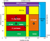Fig. 1 The XY toy model used for validation. Color code: yellow = sodium (plenum or rod followers), red = inner fuel, orange = outer fuel, green = fertile (lower axial blanket, plate in the inner core), purple = absorbers, blue = reflector. Boundary conditions: specular reflection (left), vacuum (right, top and bottom). The dashed white line encloses the regions represented in Figure 2 and Figures 4 to 8.

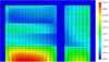Fig. 2 Uncertainty map for the R i ratios over the 748 regions of discrete description P1 (%).

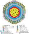Fig. 3 Loading pattern of the ASTRID reactor.

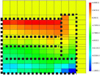Fig. 4 ASTRID reactor − Fissile + fertile partition into 132 regions − Sensitivity of the fission source distribution to the 56Fe elastic cross-section.

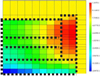Fig. 5 ASTRID reactor − Fissile + fertile partition into 132 regions − Sensitivity of the fission source distribution to the 16O elastic cross-section.

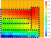Fig. 6 ASTRID reactor − Fissile + fertile partition into 132 regions − Sensitivity of the fission source distribution to the 238U capture cross-section.

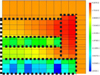Fig. 7 ASTRID reactor − Fissile + fertile partition into 132 regions − Sensitivity of the fission source distribution to the 238U inelastic cross-section.

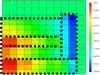Fig. 8 ASTRID reactor − Fissile + fertile partition into 132 regions − Sensitivity of the fission source distribution to the 239Pu fission cross-section.

4 Conclusions and perspectives

This review article presented two recent applications of perturbation theory, which is one of the activities Massimo Salvatores was involved into:

• some of the new possibilities offered by a coupling between a nuclear evaluation code and an advanced Monte Carlo transport code;

• how the coupling of a continuous and a discrete (multipoint) models enables calculate simply the sensitivity of the state eigenvector to multigroup nuclear data.

First, the IFP method gives promising results for nuclear parameters sensitivity calculation, reaching computation efficiency unreachable with standard perturbation method. With more complete nuclear data evaluation, the IFP method presented here will be an interesting candidate to practice integral experiment assimilation directly onto nuclear parameters, instead of the current practice on nuclear data. Such advances will considerably improve the assimilation process and its refinement. Coupling an evaluation nuclear data code and a transport code also allows direct nuclear parameter perturbations during the transport simulation, and avoids the need for ENDF format. A strong coupling between codes, the best solution to achieve this capability, is mandatory but not fully implemented yet (and not presented here).

Second, combined use is made of a multipoint description (region-to-region coupling coefficients) of the unperturbed system and of deterministic transport calculations to compute the “seed” of the perturbation investigated. Subsequently, this seed is propagated in the multipoint model. As a result, the sensitivity of the state eigenvector of the system to multigroup nuclear data is computed using simple and fast partial importance calculations, with a lower computational cost than for classical GPT calculations. This method is validated on simple toy models and then applied to the ASTRID reactor.

Author contribution statement

Elias Vandermeersch: contributed to Section 2 and conclusion Maxence Maillot: contributed to Section 3 Pierre Tamagno: contributed to Section 2 Jean Tommasi: overall responsibility of the paper, and contributed to Sections 2, 3, the foreword and conclusion Cyrille De Saint Jean: contributed to Section 2.

References

All Tables

All Figures

Fig. 1 The XY toy model used for validation. Color code: yellow = sodium (plenum or rod followers), red = inner fuel, orange = outer fuel, green = fertile (lower axial blanket, plate in the inner core), purple = absorbers, blue = reflector. Boundary conditions: specular reflection (left), vacuum (right, top and bottom). The dashed white line encloses the regions represented in Figure 2 and Figures 4 to 8.

In the text

	Fig. 2 Uncertainty map for the R i ratios over the 748 regions of discrete description P1 (%).
In the text

	Fig. 3 Loading pattern of the ASTRID reactor.
In the text

	Fig. 4 ASTRID reactor − Fissile + fertile partition into 132 regions − Sensitivity of the fission source distribution to the 56Fe elastic cross-section.
In the text

	Fig. 5 ASTRID reactor − Fissile + fertile partition into 132 regions − Sensitivity of the fission source distribution to the 16O elastic cross-section.
In the text

	Fig. 6 ASTRID reactor − Fissile + fertile partition into 132 regions − Sensitivity of the fission source distribution to the 238U capture cross-section.
In the text

	Fig. 7 ASTRID reactor − Fissile + fertile partition into 132 regions − Sensitivity of the fission source distribution to the 238U inelastic cross-section.
In the text

	Fig. 8 ASTRID reactor − Fissile + fertile partition into 132 regions − Sensitivity of the fission source distribution to the 239Pu fission cross-section.
In the text

References

- M. Aufiero, M. Fratoni, G. Palmiotti, M. Salvatores, Continuous energy cross section adjustment: a new method to generalize nuclear data assimilation for a wider range of applications, in Proceedings, M&C 2017 − International Conference on Mathematics & Computational Methods Applied to Nuclear Science & Engineering, Jeju, Korea, April 16-20, 2017, 2017 [Google Scholar]
- M. Aufiero, M. Martin, M. Fratoni, XGPT: Extending Monte Carlo generalized perturbation theory capabilities to continuous-energy sensitivity functions, Ann. Nucl Energy 96, 295–306 (2016) [CrossRef] [Google Scholar]
- M. Aufiero, G. Palmiotti, M. Salvatores, S. Sen, Coupled reactors analysis: New needs and advances using Monte Carlo methodology, Ann. Nucl Energy 98, 218–225 (2016) [CrossRef] [Google Scholar]
- P. Archier et al., Conrad evaluation code: Development status and perspectives, Nucl. Data Sheets 118, 488–490 (2014) [CrossRef] [Google Scholar]
- C. De Saint Jean, P. Tamagno, P. Archier, G. Noguere, CONRAD – a code for nuclear data modeling and evaluation, EPJ Nuclear Sci. Technol. 7, 10 (2021) [CrossRef] [EDP Sciences] [Google Scholar]
- E. Brun et al., TRIPOLI-4®, CEA, EDF and AREVA reference Monte Carlo code, Ann. Nucl. Energy 82, 151–160 (2015) [CrossRef] [Google Scholar]
- A.M. Lane, R.G. Thomas, R-matrix theory of nuclear reactions, Rev. Mod. Phys. 30, 257–353 (1958) [CrossRef] [MathSciNet] [Google Scholar]
- B. Morillon, P. Romain, Dispersive and global spherical optical model with a local energy approximation for the scattering of neutrons by nuclei from 1 keV to 200 MeV, Phys. Rev. C 70, 014601 (2004) [CrossRef] [Google Scholar]
- D. Rochman, A. Koning, Modern nuclear data evaluation with the TALYS code system, Nucl. Data Sheets 113, 2841–2934 (2012) [CrossRef] [Google Scholar]
- C. Mattoon et al., Generalized Nuclear Data: A new structure (with supporting infrastructure) for handling nuclear data, Nucl. Data Sheets 113, 3145–3171 (2012) [CrossRef] [Google Scholar]
- D.A. Brown et al., ENDF/B-VIII.0: The 8th major release of the nuclear reaction data library with CIELO-project cross sections, new standards and thermal scattering data, Nucl. Data Sheets 148, 1–142 (2018) [CrossRef] [Google Scholar]
- G. Truchet, P. Leconte, A. Santamarina, E. Brun, F. Damian, A. Zoia, Computing adjoint-weighted kinetics parameters in TRIPOLI-4® by the Iterated Fission Probability method, Ann. Nucl. Energy 85, 17–26 (2015) [CrossRef] [Google Scholar]
- Y. Nauchi, T. Kameyama, Development of calculation technique for Iterated Fission Probability and reactor kinetic parameters using continuous-energy Monte Carlo method, J. Nucl. Sci. Technol. 47, 977–990 (2010) [CrossRef] [Google Scholar]
- P. Tamagno, E. Vandermeersch, Comprehensive stochastic sensitivities to resonance parameters, in Proceedings, 2019 International Conference On Nuclear Data for Science and Technology, Beijing, China (2019) [Google Scholar]
- G. Palmiotti, M. Salvatores, G. Aliberti, Methods in use for sensitivity analysis, uncertainty evaluation and target accuracy assessment, in Proceedings, NEMEA-4–Neutron Measurements, Evaluation and Applications, Prague, Czech Republic (2007) [Google Scholar]
- B.C. Kiedrowski, Review of Early 21st-Century Monte Carlo Perturbation and Sensitivity Techniques for k-Eigenvalue Radiation Transport Calculations, Nucl. Sci. Eng. 185, 426–444 (2017) [CrossRef] [Google Scholar]
- M. Aufiero, A. Bidaud, M. Fratoni, Continuous energy function sensitivity calculation using GPT in Monte Carlo neutron transport: application to resonance parameters sensitivity study, in Proceedings, International Congress on Advances in Nuclear Power Plants (ICAPP), San Francisco, United States (2016) [Google Scholar]
- OECD-NEA, International Handbook of Evaluated Criticality Safety Benchmark Experiments, NEA/NSC/DOC(95°/03, OECD/NEA, Paris, France (2018) [Google Scholar]
- A.J.M. Plompen et al., The joint evaluated fission and fusion nuclear data library, JEFF-3.3, Eur. Phys. J. A 56, 181 (2020) [CrossRef] [EDP Sciences] [Google Scholar]
- M. Maillot, Caractérisation des effets spatiaux dans les grands cœurs RNR : méthodes, outils et études“ ( in French), PhD Thesis, Aix Marseille Université, ED 352 ( 2016) [Google Scholar]
- M. Maillot, J. Tommasi, G. Rimpault, A search for theories enabling analyses of spatial effects in highly coupled SFR cores, Proceedings, Physics of Reactors 2016, PHYSOR 2016: Unifying Theory and Experiments in the 21st Century, Sun Valley, ID, USA (2016) [Google Scholar]
- K. Kobayashi, Rigorous derivation of multi-point kinetic equations with explicit dependence on perturbation, J. Nucl. Sci. Technol. 29, 110–120 (1992) [CrossRef] [Google Scholar]
- C. Venard, The ASTRID core at the midterm of the conceptual design phase (AVP2), in Proceedings, ICAPP 2015: Unifying Theory and Experiments in the 21st Century, Sun Valley, ID, USA, paper 15275, May 03-06, 2015, Nice, France (2015) [Google Scholar]
- R. Le Tellier, C. Suteau, D. Fournier, J.M. Ruggieri, High-order discrete ordinate transport in hexagonal geometry: a new capability in ERANOS, Nuovo Cimento C 33, 121 (2010) [Google Scholar]
Cite this article as: Elias Vandermeersch, Maxence Maillot, Pierre Tamagno, Jean Tommasi, Cyrille De Saint Jean, Two examples of recent advances in sensitivity calculations, EPJ Nuclear Sci. Technol. 7, 13 (2021)
All Tables
Cross sections and angular distribution contributions to PMF001 parameters reactivity sensitivities.
Ratio of uncertainties on R i: (continuous description / discrete description), for each of the 3 discrete descriptions.
Representativeness coefficients between the sensitivity vector of R i in the continuous description and each one of the sensitivity vectors of R i in the 3 discrete descriptions.
Sensitivity of R i for position B: reference GPT values obtained by the continuous description and, between brackets, the absolute discrepancy (when it exceeds 0.001) with the sensitivity predicted using the discrete description with 384 meshes.