| Issue |
EPJ Nuclear Sci. Technol.
Volume 7, 2021
|
|
|---|---|---|
| Article Number | 4 | |
| Number of page(s) | 21 | |
| DOI | https://doi.org/10.1051/epjn/2021001 | |
| Published online | 19 February 2021 | |
https://doi.org/10.1051/epjn/2021001
Regular Article
Prediction of crack propagation kinetics through multipoint stochastic simulations of microscopic fields
1
EDF R&D, Département MMC, Avenue des Renardières,
77250
Écuelles,
France
2
EDF R&D, Département PRISME,
6 Quai Watier,
78401
Chatou,
France
* Present address: Ecole Centrale de Nantes, 1 rue de la Nöe 44300 Nantes, France.
** e-mail: This email address is being protected from spambots. You need JavaScript enabled to view it.
Received:
10
April
2020
Received in final form:
18
December
2020
Accepted:
4
January
2021
Published online: 19 February 2021
Abstract
Prediction of crack propagation kinetics in the components of nuclear plant primary circuits undergoing Stress Corrosion Cracking (SCC) can be improved by a refinement of the SCC models. One of the steps in the estimation of the time to rupture is the crack propagation criterion. Current models make use of macroscopic measures (e.g. stress, strain) obtained for instance using the Finite Element Method. To go down to the microscopic scale and use local measures, a two-step approach is proposed. First, synthetic microstructures representing the material under specific loadings are simulated, and their quality is validated using statistical measures. Second, the shortest path to rupture in terms of propagation time is computed, and the distribution of those synthetic times to rupture is compared with the time to rupture estimated only from macroscopic values. The first step is realized with the cross-correlation-based simulation (CCSIM), a multipoint simulation algorithm that produces synthetic stochastic fields from a training field. The Earth Mover’s Distance is the metric which allows to assess the quality of the realizations. The computation of shortest paths is realized using Dijkstra’s algorithm. This approach allows to obtain a refinement in the prediction of the kinetics of crack propagation compared to the macroscopic approach. An influence of the loading conditions on the distribution of the computed synthetic times to rupture was observed, which could be reduced through a more robust use of the CCSIM.
© E. Le Mire et al., published by EDP Sciences, 2021
 This is an Open Access article distributed under the terms of the Creative Commons Attribution License (https://creativecommons.org/licenses/by/4.0), which permits unrestricted use, distribution, and reproduction in any medium, provided the original work is properly cited.
1 Introduction
Stress corrosion cracking (SCC) is a major problem in the nuclear industry. It is one of the main environmental degradation phenomena affecting the materials of pressurized water reactors (PWR) [1]. In particular, the integrity of primary circuit, where flows the hot primary water (320 °C, 150 bar), is at stake since operational feedbacks revealed a potential susceptibility to SCC of various primary materials: austenitic stainless steels [2], nickel based alloys [3,4] and their weld joints [5,6]. As experienced in the past, such degradation can prompt severe consequences, hence Primary Water Stress Corrosion Cracking (PWSCC) has been getting more and more attention for the last 40 years.
SCC mechanisms require the synergistic effects of mechanical, metallurgical and environmental factors [7]. To be more specific, those effects taken into account individually may not be harsh enough to damage the material, but they jointly can lead to great damages and failure. Many SCC models have been developed so far, that can be divided into two classes. Quantitative empirical models that try to predict initiation and crack growth rate do not describe physical mechanisms, and suffer from a lack of accuracy. By contrast, models describing the possible involved physical mechanisms responsible for degradation are usually only qualitative [8,9]. EDF R&D is developing a multi-physics models of PWSCC, called the ‘local’ model [10–12]. The ambition of this model, whose main features are discussed below, is to deliver quantitative values usable for industrial end-users (e.g. crack depth vs estimated time), based on an explicit description of the different stages of SCC (incubation, initiation and propagation).
The main bottleneck of such local approaches lies in the costly sampling of experimental microscopic fields required. In particular, the experimental capture of materials variabilities such as grain morphologies, precipitates and carbides distribution is challenging [13]. One solution is to consider the microstructures as random fields, and to simulate them through statistical methods, but it is quite a tricky task. For example, the approach proposed by [14] has been focused on a heuristic of the path of the crack, based on randomly simulated microstructures using Poisson-Voronoi tessellations [15]. However, such methods lead to a binary-like space distribution, where a pixel belongs either to a grain boundary or to a grain with a specific orientation. This prevents the crack to be intragranular, yet this propagation mode is physically admissible and should not be discarded. Moreover, the experimental maps available in our work are continuous fields. Using Voronoi tessellations would presumably deteriorate this data richness. Therefore, a tesselation-type modelling is not appropriate here. Another approach, similar to the one proposed in this paper, consists in building graphs based on experimental images [16]. Fracture mechanics considerations, by means of minimizing a fracture energy criterion, are used to set the graph vertices values or weights. As interesting as this approach is, it cannot be applied to SCC since mechanics only cannot lead to damage in those conditions, as mentioned before. Finally, in the local model developed by EDF R&D and introduced before, InterGranular SCC (IGSCC) is simulated by an explicit local coupling between mechanical, oxidation and fracture parameters. It is assumed that IGSCC propagation may occur when the local opening stress, acting on a weakened oxidized grain boundary [17], reaches a critical value [18,19]. As a result, realistic trends were reproduced on an aggregate of few grains (~30). Nevertheless, it was revealed by [20] that the main limitation of such an approach is the prohibitive computational time, as the oxidation-mechanics coupling requires accurate successive refinements of the mesh where the oxidation occurs (i.e. 1 μm3 at the grain boundary). All those methods are then discarded for the prediction of crack propagation of structural components involving SCC.
In this paper, we propose a complementary approach where (i) the microstructure is simulated through the cross-correlation-based simulation (CCSIM) [21,22], a geostatistics-based algorithm and (ii) the kinetics of crack propagation is described asan empirical law that reproduces laboratory observations. In this approach, local parameters are still considered, but the couplingwith oxidation is not explicit anymore. More precisely, the oxidation is incorporated in the propagation law. As a precious gain for industrial end-users, this assumption allows to compute cracking scenarios at large scale which are closer to real industrial components. The methodology is applied to the simulation of synthetic plastic strain maps ϵp. This choice was motivated by the following considerations:
-
the plastic strain ϵp is a sensitive parameter: local plastic strain, which can be introduced in components by cold work during fabrication and installation was, found to play a significant role in both the initiation and the growth of SCC cracks in PWR primary coolant water [23], in particular where heterogeneities are significant (heat affected zone, inclusions, surfaces after machining or peening, etc.).
-
some inhomogeneities are observed in industrial components: plastic strain levels estimations in representative mock-ups of industrial components revealed a possible increase of plastic strain near fusion line of weldings.
-
some time-consuming data have been collected: ϵp cannot be directly measured, except at the surface where gauges were deposited prior to deformation. Anyway, different post-mortem techniques offer the possibility to indirectly estimate plastic strain at different scales: microhardness (HV) investigates the scale of grain aggregates, and Electron BackScatter Diffraction (EBSD) analyses, which are obtained on a Scanning Electron Microscope (SEM), can give access to local misorientations of the material. For this second method, microstructural data are processed as Kernel Average Misorientation (KAM) patterns [24] that describe the crystal misorientation fields.
In the present paper, the global approach is presented (Sect. 2), as well as the use of the CCSIM to simulate random microstructures from experimental EBSD maps (Sect. 3). Then the use of Dijkstra’s algorithm to find critical propagation paths for the crack is presented (Sect. 4). Section 5 provides conclusions and perspectives of this work.
2 The crack propagation issue
In order to validate the SCC model on lab specimens (or to evaluate it on realistic industrial components) with a global 3D view and an improved added value of data analyses, a digital tool named Code_Coriolis has been developed [25]. It consists in a finite element modeling post analysis module. The inputs are the geometry of the piece (modelled with a CAD software), the mesh of the piece, SCC models, and the boundary conditions (surfaces in contact with water and parameters of water). From these information, the tool computes the most probable path of the crack, and can display several outputs: a 3D map of crack initiation probabilities, a 3D view of the crack path and the kinetics of the crack propagation (crack depth versus time), etc.
Figure 1 summarizes the principle used in Code_Coriolis to compute the propagation of a crack: at instant t, the crack tip is at a givennode, and its neighbouring nodes are questioned (Fig. 1b). Through mechanical calculations (i.e. the maximum crack propagation speed between two nodes), the code determines the most critical node to which the crack can move (Fig. 1c), then the crack advances to this node (Fig. 1d). The process is repeated at instant t + 1 and so on, thus the crack propagation path can be determined. In the current version of Code_Coriolis, only macroscopic parameters, such as FEM outputs (stress and strain fields) are used. Thus, it uses coarse meshes which do not account for the ‘local’ model that relies on microscopic behaviour of the grain boundaries. This work aims at linking the local models with the microscopic behaviours, and proposing a new propagation criterion that gives the possibility to estimate the time to rupture of the material while takinginto account the microscopic properties. Note that the microscopic behavior itself depends significantly on microscopic properties such as grains joints and their distribution, which vary within the same material. This work accounts for the influence of microscopic inherent uncertainties (or variability) by introducing a probabilistic estimate of the time to rupture.
For a better understanding of the benefit of a change of scale, let us consider a toy example, as presented in Figure 2. The two upper figures are KAM maps (details in the next section), that are assimilated to stress maps for the sake of simplicity; below are the respective histograms of their pixel values. Suppose at this point that the code must choosebetween two nodes corresponding to the two maps, then it computes the two propagation times t. Using the macroscopic criterion presented, the right map would be chosen since it has a greater mean stress, hence a lower propagation time. However, the left map shows a relatively continuous path of high stress (red dash line), which is indeed high enough to allow thepropagation of a crack faster than on the other map. In other words, the left map is characterized by higher stresses at connected grain boundaries, hence has a crack path which is more critical than the right map.
The proposed approach can be divided into two sequential steps, the second using the results of the first. This work is presented inthe order given below:
- 1.
simulate random KAM maps from training images obtained through EBSD. The purpose is to generate synthetic maps that will be used to compute fracture paths, using an algorithm of geostatistics: the CCSIM. These simulations will be validated thanks to a criterion comparing their density probability function to that of the training image, namely the Earth Mover’s Distance.
- 2.
propose a new method to compute kinetics of cracking at microscopic scale, that will support the advantage of the change of scale. By computing the critical cracking path of an experimental map and its synthetic simulations, a refinement of the computation of the time to rupture of the piece against the actual calculus at macroscopic scale is expected.
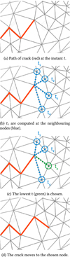 |
Fig. 1 Scheme of the computation of the advance of the crack in Code_Coriolis. |
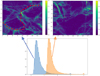 |
Fig. 2 Illustration of the benefit of the reduction of scale in the choice of the direction of propagation of the crack. Here, the right map exhibits a higher mean stress, but the left one shows a critical path of high stresses that goes through the map (dots). |
3 Simulation of stochastic microstructures
Random fields simulation is a major research topic in many fields (see for example a review in [26]). It has raised a particular interest in geostatistics, which is the analysis and modelling of phenomena using spatially localized data. In this field, the Gaussian random models are particularly useful and easy to manipulate. Once the statistical parameters (mean, variance, theoretical covariance or variogram, etc.) obtained, it is possible to simulate random fields through classical methods such as the direct simulation [27], the turning bands methods, etc., most of which are detailed by [28].
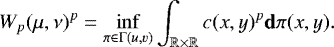
For this work, one of the objectives is to be able to simulate random fields which reproduce grain boundaries. Indeed, all the previously mentioned methods do not allow the simulation to satisfy this spatial criterion. For example, from the simulation of Figure 3 which results from the identified periodogram used by [29], one can see that the realization of the random field (left) does not exhibit the grain morphology, as does the FEM result utilized as the training image (right). As a second example, Figure 4 gives the result obtained by applying a classical geostatistical approach dealing with Gaussian random models (see for example [30]). As the initial data (shown in Fig. 4a) are far from Gaussian, the approach consists in first transforming the variable values into data which follow a Gaussian distribution (step called “Gaussian anamorphosis”), then to identify the best models for the horizontal and vertical covariances. Simulations of Gaussian data following this theoretical anisotropic covariance model can then be obtained by any of the previously mentioned methods. Finally, a simple inverse Gaussian transformation of each of these simulations allows to obtain simulations for the initial variable. By comparing Figures 4a and 4b, one can conclude that the length scales of the heterogeneities are well reproduced, but the microstructure appears to be stringy. Use of tessellation approaches allows the capture of the microstructure morphology, but in return is balanced by the challenge of capturing the data richness of a continuous random field, as analyzed in the introduction.
In this section, the type of data used (KAM fields) is presented first, as well as an algorithm formerly developed for geostatistics applications: the CCSIM. After a brief explanation of its principle and its input parameters, its application on the KAM maps is developed. To assess the quality of a realization, the use of a well known metric is proposed: the EMD (Earth Mover’s Distance), in order to compute the distance between the histograms of the training image and the simulation. The results are discussed and perspectivesare drawn in the end.
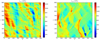 |
Fig. 3 Simulation of a stress field using the identified periodogram (left) and a FEM output utilized as the training image for the left one – extracted from [29]. |
 |
Fig. 4 (a) Example of a real microstruture to be modelled and simulated. (b) Example of a simulation coming from a Gaussian geostatistical method applied on data in (a). |
3.1 Training dataset and algorithms
3.1.1 Training dataset
The data used in this work are KAM (Kernel Average Misorientation) maps, and are obtained through EBSD (Electron Back Scatter Diffraction). KAM is a value representing the local misorientation between a pixel and its neighbours. The KAM map commonly exhibits a greater misorientation at grain boundaries than within the grains [31]. This is due to the difference in the crystallographic orientations of neighbour grains and their deformations under loading effects.
The data type studied in this work are KAM maps, where each coordinate is the KAM value at the given pixel on a 2D Cartesian grid. Figure 5 presents the training map obtained at the macroscopic strain level ϵ = 12%, displayed as an image for a better understanding of the physical interpretation of the parameters. One can see that the high values of KAM are concentrated at the grain boundaries, as expected.
The training dataset consists of 13 KAM maps of size 500 × 500, each realized at a different macroscopic strain ϵ ∈{0%, 1%, …, 9%, 10%, 12%, 15%} during a in situ tensile test. Each map was obtained by scanning the same zone in the material, one at each increment of deformation.
 |
Fig. 5 Training KAM map at ϵ = 12%. |
3.1.2 Algorithms
Developed in 2012 by [21], the CCSIM is a geostatistical algorithm and, more precisely, part of the multiple point statistics approaches [32]. It scans the training image (TI), looking for matching patterns, and stitches together these patterns in a blank image. Its main feature is the overlapping based stitching, as shown in Figure 6, extracted from [22]: each new block of pixels overlaps the one (or ones) already pasted in the blank image, and a cut following a continuous boundary that minimizes the error between the two images in the overlap region is realized (more details in Appendix A.2).
Algorithm 1 is based on the one proposed by [22], and presents the main steps of the CCSIM. The main variables are explained hereafter (others are used in the code distributed on-line by Tahmasebi)1 :
-
TI: training image, it is the reference from which all the blocks of pixels are picked.
-
T: size of the template that is being picked in the TI and pasted on the simulation grid. The same T is applied to both horizontal and vertical directions of the template.
-
OL: size of the overlap region (see Fig. A.2).
-
max_c: number of matching patterns of the TI from which one is randomly picked.
-
nreal: number of realizations to compute.
| Algorithm 1 CCSIM | |
|---|---|
| 1: | procedure ccsim(TI, T, OL, max_c, nreal) |
| 2: | for each realization ireal = 1 : nreal do |
| 3: | path ← define a raster path in the realization, which direction varies between realizations (Fig. 6: the path goes from bottom left to top right) |
| 4: | for each location u in the TI along path do |
| 5: | OLu ← extract the overlap region of size OL at the location u of the current realization. OLu can be the existing block on the left (Fig. 6A), on the bottom (Fig. 6C) or both (Fig. 6D). |
| 6: | CC ← calculate cross correlation between the newly defined overlap region OLu and TI |
| 7: | cand_loc ← Sort CC by decreasing order, and keep only the first max_c elements |
| 8: | loc ← randomly pick an element in cand_loc |
| 9: | real(u) ← assign the block consisting of loc completed with its neighbouring right/upper block of size (T-OL) (total size sizeT) at the location u in the realization (e.g. from Figs. 6C to 6D: loc completed by its upper block of size (T-OL)) |
| return all realizations | |
The most important parameters of the CCSIM are T and OL, respectively the template size and the overlap size. Great variations in quality can occur with minor variation of T and OL. Reference [33] recommends to use an OL that is between a third to a quarter the value of T. Therefore, OL is set to  as a first approach.
As detailed in the results, there is no a priori rule that helps defining T, so the CCSIM is run with different values of T that cover the minimum size computable (i.e. T = 20) to the maximum size (T = 230), on a 500 × 500 image. Once the realizations are obtained, their quality must be assessed not only through visual inspection (of the grain morphology) but also using a statistical criterion based on the pixel values. The objective is to retrieve a general rule for choosing the value of T, ideally relying on a physical parameter such as the grain size, the training image size, etc.
Using the CCSIM, a total of 16900 synthetic maps were generated: 1300 simulations were realized for each experimental map at the 13 different deformation levels (ϵ ∈ {0%, …, 15%}). In each batch of 1300 maps, 100 maps were simulated for each T and OL such as:
![Mathematical equation: \begin{align*} (T,OL) \in &\ \{(20,8), (30,10),(40,14),\ldots,(100,34),\\[4pt] &\ (120,40), (150,50), (200,68), (230,78)\}. \end{align*}](/articles/epjn/full_html/2021/01/epjn200011/epjn200011-eq2.png)
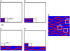 |
Fig. 6 Scheme of the CCSIM (courtesy of P. Tahmasebi). From A to D, the blank simulation is filled block by block, all extracted from the training image E. Each new block patched is randomly picked among a definite number of matching patterns. |
3.1.3 Validation of the simulations
One of the objectives of MPS algorithms such as the CCSIM is to obtain realizations that resemble the training image, but are not verbatim copies. Reference [34] uses the terms within variability and between variability to assess respectively the similarity between the training image and one realization, and between two realizations based on the same training image. To infer the quality of a CCSIM-issued simulation, two methods are used here: first the overall aspect is visually inspected, then it is proposed to compare the histograms of both the training image and the simulation. Even though apparently not robust, one must keep in mind that a visual inspection remains one of the most used methods to assess the validity of the simulations [35]. Several metrics and dissimilarity functions have been proposed for the past three decades [36,37], each comparing different parameters. The first proposals were bin-by-bin metrics, such as the Minkowski-Form distance, or the Kullback-Leibler divergence, but they do not account for cross bins information, and are sensitive to bin size [36]. Through an adaptation of the Earth Mover’s Distance (EMD, also known as the first Wasserstein distance), [36] were able to propose a new metric that often accounts for perceptual similarity better than other previously proposed methods. The idea is to use the EMD in order to define a scalar criterion that would account for an observer-based sense of the quality of the realizations (i.e. a low distance between the simulation and the training image would mean an acceptable quality). The mathematical definition of the EMD is presented in Appendix A.3.
In what follows, the terms “EMD” or “Wasserstein distance” are indifferently used to refer to the distance computed by scipy (Appendix A.3, Eq. (A.4)).
3.2 Results
Let us introduce some examples of realizations that show the different cases one can face using this algorithm. The following three figures (Figs. 7–9) show the 500 × 500 training image (which is a part of the experimental map realized at ϵ = 12%) next to 500 × 500 simulations.
The size of the simulations was limited to 500 × 500 for computational efficiency of the shortest path (see Sect. 4). Figure 7 depicts a case where visual inspection would qualify the simulation as a good reproduction of the training image’s morphology. Indeed, the grain structure seems random regarding to the training image, and no specific part could be spotted as being qualified of low quality. The EMD for this realization is EMD = 0.087.
As one can see with the orange circles in Figure 8, a pattern is repeated at least 6 times in this simulation. However, one can still observe a grain structure, but this repetition of pattern could lead the observer to naturally classify this type of realization as medium, compared to the high quality one. The EMD for this realization is EMD = 0.048. Note that the EMD for the medium quality realization is smaller than that for the high quality realization.
Finally, Figure 9 presents what could easily be considered as a low quality simulation, for it barely exhibits a grain morphology: no highly continuous deformed zones (i.e. grain boundaries) can be seen, and the field is quite homogeneous. The EMD for this realization is EMD = 0.26, which is significantly superior to the EMDs of the two previous examples (high and medium qualities).
It must also be emphasized that the medium and low quality simulations have been realized with the exact same input parameters, and come from the same run of the CCSIM. In fact, no set of parameters produced a 100% of high qualitysimulations, there are always simulations of medium and low quality in the 13 batches of 100 realizations (and in any other tried and not studied in this work). So as to see the effect of the input parameters T and OL on the EMD, the distribution of the EMD versus T ∈{20, …, 230} is displayed in Figure 10, for ϵ = 12%. The same plot has been realized for all the other levels of deformation, but are not shown in this study for the sake of conciseness.
Both Figure 10 (in addition to all the 12 other plots at the other levels of deformation not shown here) and Figure 11 show some correlation between T and the EMD of the realizations: at very “low” T, i.e. T∈{20, 30}, the mean EMD and variance are low, but the quality is visually unsatisfying as the structure is relatively homogeneous (Fig. 11b). In the range of medium T, i.e. T∈{40, …, 80}, the mean EMD is stabilized around roughly 0.12, but the dispersion increases significantly. It is however in this range that the realizations satisfy the visual inspection the most (Fig. 11c). For higher T i.e. above 100, the mean EMD first increases to a maximum (around 0.23 for T = 120), then decreases to 0.14. In this range, the dispersion is also high, and the visual aspect is poor: nearly all the realizations in this range show either pattern repetition (Fig. 11d) or no pattern at all (Fig. 9b). Finally, the plots of the EMD vs T for all the 13 macroscopic maps (not shown here) highlight that the mean EMD and its dispersion greatly increase with the load: at ϵ = 1% the mean EMD is around 0.05, and it goes up to 0.25 for ϵ = 15%.
The CPU times required for one realization varied between roughly 3 seconds for T ≥ 60 up to less than a dozen of minutes for lower T.
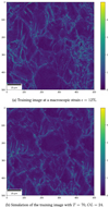 |
Fig. 7 High quality simulation example – EMD = 0.087. |
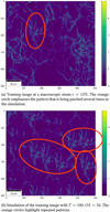 |
Fig. 8 Example of the issue of the repetition of patterns in the simulation – EMD = 0.048. |
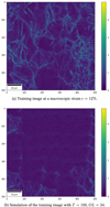 |
Fig. 9 Low quality simulation example – EMD = 0.26. |
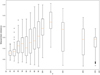 |
Fig. 10 Evolution of the EMD for 100 realizations of the 500 × 500 training image at ϵ = 12% with T varying in {20, 30, …, 100, 120, 150, 200, 230} and OL set to a thirdof T. |
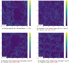 |
Fig. 11 Examples of impact of T and OL on simulations’ quality – (T, OL) ∈{(20, 8), (70, 24), (200, 68)}. |
3.3 Discussion
The first thing to discuss is the use of the term “visual quality” employed in the previous part. They obviously lead to a very subjective and observer dependent approach of the problem. However, since simulation of EBSD maps has not been done yet (to the best of authors’ knowledge), the tools available in geostatistics (where the CCSIM comes from) were used as a first approach. It could, for example, have been possible to get interested in connectivity metrics, as proposed by [38], and compute the connectivity function τ(h) (h here is the lag vector), but its computation time is prohibitive (several hours for a single map). In this work, EMD was proposed as a criterion for being quite intuitive and fast to compute. It is a scalar criterion that makes sense in itself, as distances are indeed intuitive and genuinely understandable. However, its simplicity comes with a cost as shown previously: it cannot assess perfectly the quality of a simulation. Indeed, due to its simplicity, this metric does not transport enough information in the present case, as it isbased on a 1-dimensional arrays comparison, whereas the data used in this work are 2-dimensional arrays, with spatial variability. Even though this distance can fairly eliminate the poor simulations (e.g when EMD ≥ 0.20), it cannot properly give full account of the pathologies previously described. Indeed, some simulations exhibiting patterns repetition have a low EMD (below 0.05). Yet, using the EMD to find a range of suitable input parameters is an interesting lead: Figure 10 shows a plateau in the range 40 ≤ T ≤ 80, on which the mean EMD is stabilized, and corresponds to a better proportion of high quality simulations. The recommendation that can be drawn from this work is to use 60 ≤ T ≤ 80, OL to a third the value of T, in order to maximize the occurrence of good simulations. Yet it is certain that each training image is specific, and that there is no global rule leading to the prior determination of T and OL. No relationship was found when trying to link the grain size (which is an accessible parameter) to T. This could be due to the fact that the process of determining the grain diameter relies on the assumption that the grains are circular (see Appendix A.1), whereas T and OL are square patches.
The training images used here are well suited for the exercise, as they exhibit a fairly smooth microstructure: the deformations are concentrated at the grain boundaries, and there are no complicated behaviours such as textures for instance. It is probable that using maps with complex behaviours as training image would lead to very variable results, e.g maps with some sparse large carbides or large secondary phases, incoherent with the matrix. It is supported by the fact that the EMD tends to augment with the macroscopic strain: in other words, the coarser the grain boundaries (i.e. the more deformations are concentrated at the grain boundaries), the more difficult it is to produce synthetic maps with a low EMD. More generally, any field exhibiting very local but pronounced behaviours would be hard to simulate without the use of conditioning data. The EMD would require an additional information in order to be fully useful here, e.g. periodograms and variograms [29], or energy distance [39].
Finally, the performances were in accordance with the literature, yet it could be interesting to have a deeper look at the multi-scale approach of the CCSIM, that permits a diminution of the CPU times [22], especially when one would apply this method to 3D problems.
4 Computation of crack propagation time
The multi physics aspect of SCC mechanisms make them challenging issues for the scientific community of mechanical engineer and corrosion scientists. Besides the aforementioned local SCC model [25], the present study shares some similarities with the work of [40], who tried to model SCC mechanisms in a Ni based alloy (Inconel 600). Through a phase field approach, a modelling of the diffusion coefficient and a prescription of displacements thanks to an image processing based on digital image correlation, their results exhibited great agreements with the experiments (i.e. prediction of crack morphology). One of the main differences with the present study is that the work is done at a microscopic scale, where the grain morphology itself is assumed to influence the kinetics of crack propagation.
In this section, first the computation of the local strain from KAM maps is explained, and then the use of empirical laws to determine the maximum crack speed locally. Knowing the strain at each pixel, this relationship assigns a speed of crack propagation to every pixel. Second, Dijkstra’s algorithm (which was formerly made for oriented graphs [41]) is adapted to the present case: by defining the adjacency matrix of an image, it is possible to compute the critical crack path going through it, i.e. the crack with the lowest travel time (or equivalently the highest overall speed), going from the left edge to the right edge. A graphical summary is proposed below (Fig. 12) Definitions and parametrization of the problem are presented hereafter.
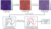 |
Fig. 12 Graphical summary of the steps used to compute the crack propagation time. |
4.1 Constitutive equations
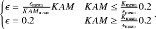
The determination of strain fields using EBSD mappings techniques has been studied in the past two decades [42,43]. Even though promising results were obtained, there is no direct relationship between the KAM and the strain ϵ at the pixelscale [31]. But since the computation of the crack speed requires the strain ϵ, a thresholded relationship between the KAM value and the local strain (Eq. (1), Fig. 13) is assumed:
 (1)
(1)
Hence ϵ varies between 0% and 20%. This relationship is the simplest the authors could define between the KAM and the local strain, as no study has been able to propose any more relevant alternative yet. Equation (1) ensures a mean strain on the maps close to the experimental, as well as a maximum strain of 20%, which correlates the experimental data.
As introduced in Section 2, the computation of the propagation time of cracks is made through the implementation of empirical laws whose shape and coefficients have been determined using experimental data. SCC being a multi-physics phenomenon involving corrosion and mechanics, the empirical law is a product of functions, each handling a specific part of the physics of the problem, e.g corrosion, kinetics, etc. The main law is the one that computes the maximum crack speed ȧmax, in μm h−1:
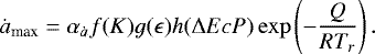 (2)
(2)
The different terms in (2) are listed and explained below:
-
f(K): K is the stress intensity factor as defined in equation (3), and f is a function inferring a thresholded behaviour (Eq. (4)). It implies that barely no propagation occurs under K0. We have:
 (3)
(3)
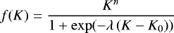 (4)
(4)
-
h(ΔEcP): ΔEcP is the electrochemical potential determined using a Nernst-like law (Eq. (5)). The solution chemistry in contact with the polycristal is modeled in this function, which takes as input the concentration in dihydrogen in the water, aswell as the temperature. The function h has been empirically determined by fitting data from laboratory experiments conducted in autoclaves in representative primary water (around 320 °C and 150 bar) (Eq. (6)). We have:
![Mathematical equation: \begin{equation*} \UpDelta EcP = 1000 \frac{R. T_r}{2. F}\ln\left(\frac{[H_2]_{test}}{[H_2]_{Ni/NiO}}\right)\end{equation*}](/articles/epjn/full_html/2021/01/epjn200011/epjn200011-eq7.png) (5)
(5)
![Mathematical equation: \begin{equation*} h(\UpDelta EcP) = 1 + 3.604\exp\left[-\frac{1}{2}\left(\frac{\UpDelta EcP + 11.33}{43.36}\right)^2\right]\end{equation*}](/articles/epjn/full_html/2021/01/epjn200011/epjn200011-eq8.png) (6)
(6)
-
 : Arrhenius-like law inferring the thermodynamic aspect of the process. As the temperature increases, so does the crack speed.
 -
g(ϵ): ϵ is the plastic strain in the material. It is easily computed by Finite Element Analysis at a macroscopic scale, however it is still quite difficult to assess the local strain at a microscopic scale from only KAM maps. ϵ is computed from the KAM maps using equation (1). The function g depends on the piece studied, the form proposed is:
 (7)
(7)
Since not all the laws have been fitted with the same accuracy, only the most studied and referenced ones in the french nuclear industry are used, which details are given in equation (8) and Table 1:
![Mathematical equation: \begin{equation*} \begin{array}{rl} \dot{a}_{\textrm{max}} = &\alpha_{\dot{a}}\frac{K^n}{1+\exp\left[-\lambda(K-K_0)\right]}\epsilon^{3.6}\\ &\left(1 + 3.604\exp\left[-\frac{1}{2}\left(\frac{\UpDelta EcP + 11.33}{43.36}\right)^2\right]\right)\\ &\exp\left[-\frac{Q}{RT_r}\right]\end{array}. \end{equation*}](/articles/epjn/full_html/2021/01/epjn200011/epjn200011-eq11.png) (8)
(8)
The speeds are computed in μm h−1, but they may be displayed relatively to a reference time (i.e. the time to rupture of the training image) when possible.
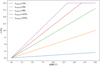 |
Fig. 13 Plot of the law that transforms the KAM into the deformation ϵ. The linear part is fitted on the macroscopic strain ϵ0 and the maximum is set at ϵmax = 20%. |
4.2 Algorithms
Once the strain maps are computed from the KAM maps, they are used to predict the most critical crack path: applying equation (8) to a deformation map leads to a map of crack speed (or velocity map) and, since the goal is to obtain the most criticalcracking path, it is equivalent to finding the path with the lowest propagation time between two points/surfaces, so propagation times must be defined. For the sake of simplicity, only the critical path between the left edge and the right edge of the maps is computed.
To achieve this goal, Dijkstra’s algorithm was adopted. It is commonly used for the computation of the less expensive path of weighted and oriented graphs [41]. Its principle is very basic as it calculates, starting from a given node, the cheapest path (in terms of weights) to a target. A graph is an ordered pair G = (V, E) comprising a set V of nodes and a set E of edges. Elements of E are 2-element subsets of V, linking 2 nodes. It is called oriented and weighted when its edges have orientation, and a weight is assigned to each edge. It can be represented by an adjacency matrix M, which is a square matrix where the coefficient Mi,j represents the weight of the displacement from the node i to the node j. The focus of this paper is on general oriented and weighted graphs, but several other examples of specific graphs can be found in [44].
To apply Dijkstra’s algorithm here, the first step is therefore to define the graph G and the adjacency matrix A corresponding to the image.. Let I denote the image, represented as a NxN matrix, and Ii,j the value of the pixel of I located at the row i and the column j. In this case, Ii,j is the speed of the region covered by the pixel (i, j). As Dijkstra’s algorithm computes the shortest path, the idea is to use the time to propagate from one node to another as the weights of the edges. The nodes are defined as being located at each corner of a pixel, i.e. on a (N + 1) × (N + 1) grid, as shown in Figure 14a. Now that the nodes have been defined, the relationship between each node must be defined as well. The studied structure is an 8-connected one, meaning that each node has a maximum of 8 neighbours, which makes 9 weights to compute for each node (the weight that loops a node on itself has to be defined). The 9 weights are defined as follows (and summarized in Fig. 14b):
-
since the crack is supposed to propagate forward, a null weight is assigned to the edges that send a node backward, leaving 6 relationships to define.
-
it is assumed that the crack never stops, hence the weight {D → D} is also set to 0.
-
for the 5remaining nodes:
-
{D → B} and {D → H}: the crack crosses the pixel so it does propagate within a constant speed region, to a distance
![Mathematical equation: $\sqrt[]{2}d$](/articles/epjn/full_html/2021/01/epjn200011/epjn200011-eq12.png) . These weights are set to respectively:
. These weights are set to respectively:
![Mathematical equation: \begin{equation*} \begin{split} \{D\rightarrow B\} = \frac{\sqrt[]{2}d}{I_{i,j}} \\ \{D\rightarrow H\} = \frac{\sqrt[]{2}d}{I_{i+1,j}}\end{split} \end{equation*}](/articles/epjn/full_html/2021/01/epjn200011/epjn200011-eq13.png) (9)
(9) -
{D → A}, {D → E} and {D → G}: the crack crosses the border between 2 pixels. It has been decided to use the mean of the 2 values of the pixels, which is supported by the fact that neighbouring pixels have usually close value (continuity of the fields). The distance is the length d of the pixel, then :
-
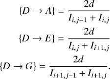 (10)
(10)
The resolution is d = 0.25μm for all the maps in this work. Now that the image has been parametrized into a graph, Dijkstra’s algorithm can be applied, whose pseudo-algorithm is proposed below in Algorithm 2.
| Algorithm 2 Dijkstra | |
|---|---|
| 1: | procedure Dijkstra(graph, source) |
| 2: | for each vertex V in graph do |
| 3: | dist[V] = ∞ |
| 4: | previousl[V] = 0 |
| 5: | dist[source] = 0 |
| 6: | Q = set of all the nodes in graph |
| 7: | while Q ≠ ∅ do |
| 8: | u = node in Q with min(dist) |
| 9: | remove u from Q |
| 10 | for each neighbour V of U do |
| 11: | alt = dist[u] + dist(u,v) |
| 12: | if alt ≤ dist[V] then |
| 13: | dist[V] = alt |
| 14: | previous[V] = u |
| return previous | |
The dataset used in this section is the same batch than the one used in Section 3: 100 realizations of the training 500 × 500 training image (Fig. 11a) for each T and OL such as:
![Mathematical equation: \begin{align*} (T,OL)\in\ &\{(20,8), (30,10),(40,14),\ldots,(100,34),\\[4pt] &\ (120,40), (150,50), (200,68), (230,78)\}. \end{align*}](/articles/epjn/full_html/2021/01/epjn200011/epjn200011-eq15.png)
The purpose here is the study of the influence of both T and OL on the times to rupture, hence Dijkstra’s algorithm was applied to the 1 300 realizations of the KAM maps at both ϵ = 2% and ϵ = 12%.
 |
Fig. 14 Parametrization of the image I, assuming that the crack only propagates forward (to the right), in order to create the graph G and the adjacency matrix A for Dijkstra’s algorithm. |
4.3 Results
First, Figure 15 presents two examples of shortest paths displayed on top of their corresponding velocity maps. It must be noticed that these two realizations could respectively be classified as high and low quality, respectively,both with a low EMD (see Sect. 3). The CPU time required to obtain the shortest path between theleft edge and the right edge of one image is around 3mn (the performances are similar for all the simulations).
Figure 16 shows the results of the application of Dijkstra’s algorithm for different realizations of CCSIM with
![Mathematical equation: \[ T\in\{20,30,40,50,60,70,80,90,100,120,150,200,230\} \]](/articles/epjn/full_html/2021/01/epjn200011/epjn200011-eq16.png)
on both synthetic (boxplots) and experimental (red line) maps, as well as the result at the macroscopic scale (green line), at two levels of deformation: 1% and 12%. Note that the two plots cannot be directly compared to each other as the references (time to rupture of the training image) are some orders of magnitude different. Several comments can be made: first, the figures highlight the difference inthe times to rupture for the two approaches (micro and macro). In fact, a factor 9 is observed between the time to rupture using Dijkstra’s algorithm on the experimental map and the one at the macroscopic scale, and a factor between roughly 1.5 and 10 for the synthetic maps and via the macroscopic approach at ϵ = 1%. The same remark can be made for the higher strain. Second, the synthetic maps are statistically overestimating the time compared to the experimental maps, with only a few realizations underestimating it, except at ϵ = 12% and for T ∈{60, 70, 80}∪{200, 230}, where the results are well distributed around the reference. Finally, one can again see the pronounced dispersion in the results issued from the synthetic maps: there is a factor of more than 5 between the lowest and the highest time at T = 120, and a factor of more than 2 at T = 30, for the two levels of strain.
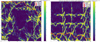 |
Fig. 15 Shortest paths (red dots) displayed on top of the velocity maps for two realizations of the CCSIM issued from the map at ϵ = 12% - left: T = 60, OL = 20, right: T = 230, OL = 78. |
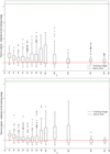 |
Fig. 16 Times to rupture of 1 300 realizations for varying T and OL, at a macroscopic strain ϵ = 1% (top) and ϵ = 12% (bottom) alongside with the time to rupture of the corresponding training image, and the macroscopic time. The times are displayed relatively to the one of the training image. |
4.4 Discussion
The results depicted in Figure 16 show the benefits of the microscopic approach: there is a factor of at least 3 between the microscopic and macroscopic approaches for the 2 levels of deformation. For T ∈{60, 70, 80} and ϵ = 12%, the times to rupture are well distributed around the one of the training image. This demonstrates the fact that the synthetic maps can actually be used to take into account the effect of microscopic variability –(e.g. when the grain morphology might differ from the reference experimental material) in the times to rupture. In some extreme cases, when the morphology changes significantly, the time to rupture might differ considerably from the reference value. Using the synthetic maps, one is not limited to a deterministic estimation of the rupture time, but can obtain a probabilistic description of this quantity. In order to reduce the effect of a single training image, one might use more experimental training images from the same material under the same loading conditions.
At lower macroscopic strain (ϵ = 1%), the results are not as good and this, for any T, which implies an effect of the strain level on the quality of this approach. It does not corroborate the results shown in Section 3, which exhibited the influence of the load on the EMD: as the load increases, so does the distance between the training image and the realizations (Fig. 10). It could confirm the previous conclusion that the EMD is not a perfect criterion to validate the simulation.
Some works remain to be done in order to reinforce this new method, as a sound relationship between the KAM and the strain ϵ (Eq. (1)) has not been found. Indeed, it is assumed here that the maximum strain is ϵmax = 20% for any load (from 1% to 12%), which is a strong assumption. Moreover, the relationship used here implies the existence of “clusters”of high velocity that get larger with higher macroscopic strains as shown in Figure 15, but no evidence of this phenomenon was found in this study. The GND (Geometrically Necessary Dislocations), which is an estimation of the density of dislocation in the material, seems to be a promising parameter to obtain the aforementioned local strain maps [45,31]: it is more physical than the KAM, hence it should lead to a more robust estimation of the local deformation.
It is worth noting that this approach only computes the shortest path on a fixed configuration of the material, i.e. it proposes a virtual crack path. The changes in mechanical and material properties (e.g. local Young’s modulus, strain, stress,..) in the surrounding area of the crack tip, as it is the case for example during cyclic loading [46,47], are not taken into account.
As this method is to be implemented in Code_Coriolis, it is assumed that the CPU times must not be too important. With an average of 3mn per simulation to compute the time to rupture between the left and the right edges of a 500 × 500 image, it is for now too high of a cost to be used like this, especially since the final goal is to draw a sample of several synthetic maps and compute their time to rupture to obtain a probabilistic distribution. Several points could lead to an improvement of the performances: first, only the shortest paths between the left and right edges of the image were considered, i.e. the algorithm is forced to search in a set of 251001 paths (501 nodes on the left, 501 on the right). Yet having a prior knowledge of where is the crack starting would lead to greatly reduced CPU times since there would be only one source.
Another idea is to compute the shortest path between reduced sets of sources and targets, assuming that this path will overlap the true critical path after a small number of pixels. It is believed that this estimator should not be too far from the shortest time for the path sought (computed between the left and right edges), but it would always overestimate this targeted value (which is the minimum of all the possible times). To ensure that this method is worth the try, Dijkstra’s algorithm was run on a single map with a varying number of sources and targets for each run, and the CPU times were stored for each computation. The results are shown in Figure 17, which exhibits a linear relationship between the number of sources and the CPU time, with times going from less than 40s to more than 2mn. It appears that the method proposed above could be interesting in order to reach reasonable CPU times.
A second point is to have a look at other pathfinding algorithms such as A* (A-star), which is supposed to be more efficient than Dijkstra [48]. A-star which is an informed search algorithm uses an evaluation function to guide the selection of nodes. It maintains a tree of paths originating at the start node and extends those paths one edge at a time. At each iteration, A-star determines the paths to be extended and prunes away significant number of nodes that an uninformed search algorithm like Dijkstra would explore. The selection is based on the evaluation function f(n) = g(n) + h(n) where g(n) represents the cost of the path from the starting point to the node n and h(n) is a heuristic function estimating the cost of the path from node n to the target point. If the heuristic function never overestimates the actual cost to get to the goal, A-star algorithm will return a least-cost path from start to goal. The time complexity of A-star algorithm depends on the heuristic function, which is problem-specific. However, due to the fact that only a selected number of paths is explored, A-star provides the optimal path faster than Dijkstra when the correct heuristic is chosen.
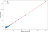 |
Fig. 17 CPU time for Dijkstra’s algorithm vs the number of sources and targets for the experimental map at the macroscopic strain ϵ = 12% - 500 × 500 image i.e. 251 001 (=501 × 501) nodes in thecorresponding graph (with the parametrization assumed in this work). |
5 Conclusion and perspectives
In this paper, it is shown that using microscopical fields permitted a refinement in the prediction of the propagation of a crack into a metallic material. This was rendered possible thanks to a two-step approach that takes into account the microstructural heterogeneities (e.g concentration of deformation at grain boundaries) in the SCC models, instead of using global macroscopic parameters. As a result, one obtains a probabilistic description of the time to rupture, which is considerably more informative than a single deterministic estimation.
Using the CCSIM to simulate microstructures has been demonstrated possible and provides promising results. However, it has been shown that more work is required in order to assess the quality of the synthetic maps: the EMD proved to be insufficient by itself. A solution is that the EMD be completed by additional criteria that can infer the spatial heterogeneities of the random fields studied here. Variograms, periodograms, etc. seem interesting leads, but computing those parameters on fields as large as the ones used in this work (at least 500 × 500) is expensive. A general indicator of the value a priori of the input parameters of the CCSIM (T and OL) is yet to be found.
The computation of the times to rupture using Dijkstra’s algorithm was found to be promising. Indeed, through a correct parametrization of the studied random field into a graph, it could be possible to apply this method to numerous fields: temperature, chemistry, mechanics, etc., which makes this method quite generic. Yet, one must keep in mind that a strong hypothesis lies at the base of this approach: a sound relationship between the KAM and the deformation ϵ at the microscopic scale, that is of the utmost importance, has yet to be determined. This is why the results must be interpreted with that information in mind, even though they are encouraging. Once this relationship is scientifically more robust, one will be able to make proper comparisons between this new microscopic approach and the macroscopic one.
The perspectives for this work can be summarized as follows :
-
the determination of the local deformation ϵ should be studied, as it constitutes the basis of the approach. It is more likely to be related to the GND than to the KAM, but both fields are easily obtained with EBSD.
-
it would be interesting to find an indicator that could give a value a priori of the input parameters of the CCSIM, so as to lead to a higher proportion of good simulations without having to try a lot of combinations beforehand. Moreover, the influence of OL has not been studied, since it was set to a third of the value of T. To go further, running new simulations with different values of OL is advised, as the recommendations given by [33] may not be suitable for this application.
-
as for now, the implementation of the approach is also limited by its CPU time. The main drawback of Dijkstra’s algorithm is its computational cost, which makes it the bottleneck of the whole process. Yet the conclusion regarding this aspect is optimistic, as it has been shown that this could be dealt with by using more powerful algorithms such as A* [48], or through a smart choice of the sources and targets.
-
the full potential of the CCSIM has not been exploited, and it could be interesting to have a look at the multi-scale approach developed by [22], or other pattern-based methods such as a conditional probability formulation [49] or the HYPPS algorithm [49,50]. It could also allow fast simulations of microstructures in 3D.
Programming tools
The main programming tool used for the simulation of the microstructure is MATLAB 2017b, with the toolbox Image Processing useful for its function xcorr2.m. It is significantly faster than its Python equivalent correlate2d(x,y) from the library scipy.signal. As mentioned above, the EMD is computed with the function scipy.stats.wasserstein_distance. Note that other packages dedicated to optimal transport can be found (e.g POT), but optimization of computation times is not the focus of this work.
The main tool used to deal with the simulation of the crack paths is Python 3.6: the definition of the adjacency matrix was realized with the function dok_matrix from the package scipy.sparse.dok. It builds a sparse matrix that is to be parametrized by the user. Dijkstra’s algorithm is also available on scipy: scipy.sparse.csgraph.dijkstra. Those tools were used to find the shortest path between the left edge and the right edge of the images.
Author contribution statement
This work is the result of the Master’s internship of E. Le Mire, supervised by E. Burger, C. Mai and B. Iooss. E. Le Mire carried out the numerical implementation, performed the tests and wrote the methodological parts of the manuscript. All authors participatedto the discussion of results. E. Burger, C. Mai and B. Iooss performed scientic advisory roles and provided support through expert judgement, critical verification, proofreading and writing introductory parts of the manuscript.
Acknowledgements
The authors are grateful to the EDF R&D microscopy department, the Materials Ageing Institute (MAI), for having supplied with the KAM data. They also thank two anonymous referees for their remarks, as well as Julien Vidal for having provided his remarks on a preliminary version of this paper. Finally, the authors wish to acknowledge Thierry Couvant and Jerome Ferrari for having provided helpful opinion during this work, and Géraud Blatman for his preliminary studies on the subject.
Appendix
A.1 Experimental data – supplementary material
Figure A.1 presents the distribution of the grain diameter of 7 of the 13 experimental maps. In order to determine those values, the grains are likened to circles, and sorted in 20 ranges of values, hence the interpretation of the graph should be realized with that information in mind. The acquisition of the EBSD maps were led on a Tescan Mira 3 SEM, which parameters are shown in Table A.1.
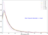 |
Fig. A.1 Fitted distribution of the grain diameter (μm) of some experimental maps. 20 bins were used for the fit. |
Acquisition parameters of the experimental EBSD maps.
A.2 Minimum error boundary cut
As presented in the Section 3, the CCSIM goes through a step to smoothen the stitching of two images side by side. The idea is to compute the error between 2 overlapping regions, and to calculate the cumulative minimum error line by line. It is then possible to create a continuous path of minimum error. Algorithm 3 (adopted from [33]), presents how a 2D vertical smooth stitching is done. It is easily applied to an horizontal cut. Figure A.2 summarizes this process on an example.
| Algorithm 3 Minimum error cut | |
|---|---|
| 1: | procedure mincut Two overlapping patching B1, B2, with overlapping areas B1OV, B2OV |
| 2: | Define an error surface e = (B1OV− B2OV)2, size (p,m) |
| 3: | Compute the cumulative minimum error along the cutting direction : |
| 4: | for each row i in e (i = 2,..p) do |
| 5: | for each column j in e (j = 1,..m) do |
| 6: | Calculate the cumulative minimum error E using the 3 closest pixels on the previous row (2 if on an edge) : |
| 7: | Ei,j = ei,j + min(Ei−1,j−1, Ei−1,j, Ei−1,j + 1); if j = 2, …, m − 1 |
| 8: | Ei,j = ei,j + min(Ei−1,j, Ei−1,j+1); if j = 1 |
| 9: | Ei,j = ei,j + min(Ei−1,j−1, Ei−1,j); if j = m |
| 10: | k ← identify the coordinate k corresponding to the entry with the smallest minimum value on the last row of E (i.e. arrival point of a path of minimum cost through the error surface) |
| 11: | min ← trace back the minimum values for each row i going backward (i = p − 1, …, 1), and each time identify the cutting path as min(Ei,k−1, Ei,k, Ei,k+1) |
| return Minimum error boundary cut | |
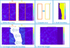 |
Fig. A.2 Stitching process: the 2 OL regions are first defined (1.), the error is then computed between these 2 regions (2.) and a continuous path of minimum error is built (3.). The 2 images are cut along this path (4.) and finally stitched together, with a smooth boundary (5.). |
A.3 Earth Mover’s distance
The EMD isactually the optimal transport distance when considering the optimal transport (or Monge-Kantorovitch) problem, which consists in finding the most efficient plan to rearrange one probability measure into another. Kantorovitch version goes as follows [37]: let (X, μ) and (Y, ν) be two probability measure spaces, π be a probability measure on the product space X × Y. Let ∏ (μ, ν) = {π ∈ P(X × Y): π[A × Y ] = μ[A] and π[X× B] = ν[B] hold for all measurable sets A ∈ X and B ∈Y } be the set of admissible transport plans. For a given cost function  where c(x, y) means the cost of moving from location x to location y, the total transport cost associated to plan π ∈∏ (μ, ν) is:
![Mathematical equation: \begin{equation*} I[\pi]=\int_{X\times Y}c(x,y)\mathbf{d}\pi(x,y). \end{equation*}](/articles/epjn/full_html/2021/01/epjn200011/epjn200011-eq18.png) (A.1)
(A.1)
The optimal transport cost between μ and ν is:
![Mathematical equation: \begin{equation*} T_c(\mu,\nu)=\underset{\pi\in\prod(\mu,\nu)}{\inf} I[\pi]. \end{equation*}](/articles/epjn/full_html/2021/01/epjn200011/epjn200011-eq19.png) (A.2)
(A.2)
More specifically, the p-Wasserstein distance is a finite metric on (X, μ) defined as in [51]:
 (A.3)
(A.3)
In practice, the function scipy.stats.wasserstein_ distance from the Scipy library is used. It is defined as follows when c(x, y) = ∣x − y∣: for two distributions u and v, the first Wasserstein distance (named EMD when p = 1) goes as:
 (A.4)
(A.4)
References
- S. Zinkle, G. Was, Acta Mater. 61, 735 (2013) [CrossRef] [Google Scholar]
- D. Féron, E. Herms, B. Tanguy, J. Nuclear Mater. 427, 364 (2012) [CrossRef] [Google Scholar]
- P. Scott, An overview of materials degradation by stress corrosion in PWRs, in EUROCORR 2004: long term prediction and modeling of corrosion, France (IAEA/INIS, 2004) [Google Scholar]
- P. Andresen, J. Hickling, A. Ahluwalia, J. Wilson, Corrosion 64, 707 (2008) [CrossRef] [Google Scholar]
- Q. Peng, T. Shoji, H. Yamauchi, Y. Takeda, Corros. Sci. 49, 2767 (2007) [CrossRef] [Google Scholar]
- L. Lima, M. Schvartzman, C. Figueiredo, A. Bracarense, Corrosion 67, 085004 (2011) [CrossRef] [Google Scholar]
- A. Turnbull, Corros. Sci. 34, 921 (1993) [CrossRef] [Google Scholar]
- Z. Zhai, M. Toloczko, M. Olszta, S. Bruemmer, Corros. Sci. 123, 76 (2017) [CrossRef] [Google Scholar]
- Z. Shen, K. Arioka, S. Lozano-Perez, Corros. Sci. 132, 244 (2018) [CrossRef] [Google Scholar]
- T. Couvant, M. Wehbi, C. Duhamel, J. Crépin, R. Munier, Development of a local model to predict SCC: preliminary calibration of parameters for nickel alloys exposed to primary water, in 17th International Conference on Environmental Degradation of Materials in Nuclear Systems-Water Reactors (2015) [Google Scholar]
- T. Couvant, M. Wehbi, C. Duhamel, J. Crépin, R. Munier, Grain boundary oxidation of nickel base welds 182/82 in simulated PWR primary water, in 17th international conference on environmental degradation of materials in nuclear power systems-water reactors (2015), pp. 25–p [Google Scholar]
- M. Wehbi, T. Couvant, C. Duhamel, J. Crepin, Mater. High Temp. 32, 1 (2015) [CrossRef] [Google Scholar]
- B. Sudret, H. Dang, M. Berveiller, A. Zeghadi, T. Yalamas, Front. Struct. Civil Eng. 9, 121 (2015) [CrossRef] [Google Scholar]
- S. Arwade, M. Popat, Probab. Eng. Mech. 24, 117 (2009) [CrossRef] [Google Scholar]
- K. Sobczyk, Probab. Eng. Mech. 23, 444 (2008) [CrossRef] [Google Scholar]
- D. Jeulin, Eng. Comput. 10, 81 (1993) [CrossRef] [Google Scholar]
- J. Dohr, D. Armstrong, E. Tarleton, T. Couvant, S. Lozano-Perez, Thin Solid Films 632, 17 (2017) [CrossRef] [Google Scholar]
- S. Bruemmer, M. Olszta, M. Toloczko, D. Schreiber, Corros. Sci. 131, 310 (2018) [CrossRef] [Google Scholar]
- G. Bertali, F. Scenini, M. Burke, Corros. Sci. 111, 494 (2016) [CrossRef] [Google Scholar]
- T. Couvant, D. Haboussa, S. Meunier, G. Nicolas, E. Julan, K. Sato, F. Delabrouille, A simulation of IGSCC of austenitic stainless steels exposed to primary water, in 17th International Conference on Environmental Degradation of Materials in Nuclear Power Systems-Water Reactors, Ottawa, CA, August 9–13 (2015), pp. 1987–2008 [Google Scholar]
- P. Tahmasebi, A. Hezarkhani, M. Sahimi, Comput. Geosci. 16, 779 (2012) [CrossRef] [Google Scholar]
- P. Tahmasebi, M. Sahimi, J. Caers, Comput. Geosci. 67, 75 (2014) [CrossRef] [Google Scholar]
- M. Hall Jr, Corros. Sci. 125, 152 (2017) [CrossRef] [Google Scholar]
- R. Shen, P. Efsing, Ultramicroscopy 184, 156 (2018) [CrossRef] [Google Scholar]
- T. Couvant, Prediction of IGSCC as a Finite Element Modeling Post-analysis, in Environmental Degradation of Materials in Nuclear Power Systems (Springer, 2017), pp. 319–334 [Google Scholar]
- M. Bilodeau, F. Meyer, M. Schmitt, in Space, Structure and Randomness: Contributions in Honor of Georges Matheron in the Fields of Geostatistics, Random Sets and Mathematical Morphology, Vol. 183 (Springer, 2007) [Google Scholar]
- P. Mukherjee, C.Y. Wang, J. Electrochem. Soc. 153, A840 (2006) [CrossRef] [Google Scholar]
- C. Lantuéjoul, Geostatistical simulations - Models and algorithms (Springer, 2002) [CrossRef] [Google Scholar]
- X. Dang, Ph.D. thesis, Université Blaise Pascal-Clermont-Ferrand II (2012) [Google Scholar]
- J.P. Chilès, P. Delfiner, Geostatistics: Modeling spatial uncertainty (Wiley, New-York, 1999) [Google Scholar]
- L. Brewer, M. Othon, L. Young, T. Angeliu, Microsc. Microanaly. 12, 85 (2006) [CrossRef] [Google Scholar]
- P. Tahmasebi, Multiple Point Statistics: A Review, in Handbook of Mathematical Geosciences: Fifty Years of IAMG, edited by B. Daya Sagar, Q. Cheng, F. Agterberg (Springer International Publishing, Cham, 2018), pp. 613–643 [Google Scholar]
- G. Mariethoz, J. Caers, Multiple-point geostatistics: stochastic modeling with training images (John Wiley & Sons, 2014) [Google Scholar]
- X. Tan, P. Tahmasebi, J. Caers, Math. Geosci. 46, 149 (2014) [CrossRef] [Google Scholar]
- B. Daya Sagar, Q. Cheng, F. Agterberg, Handbook of Mathematical Geosciences: Fifty Years of IAMG (Springer, 2018) [CrossRef] [Google Scholar]
- Y. Rubner, C. Tomasi, L. Guibas, Int. J. Comput. Vision 40, 99 (2000) [CrossRef] [Google Scholar]
- K. Ni, X. Bresson, T. Chan, S. Esedoglu, Int. J. Comput. Vis. 84, 97 (2009) [CrossRef] [Google Scholar]
- P. Renard, D. Allard, Adv. Water Resour. 51, 168 (2013) [CrossRef] [Google Scholar]
- M. Rizzo, G. Székely, Wiley Interdiscip. Rev. 8, 27 (2016) [CrossRef] [Google Scholar]
- T.T. Nguyen, J. Bolivar, J. Réthoré, M.C. Baietto, M. Fregonese, Int. J. Solids Struct. 112, 65 (2017) [CrossRef] [Google Scholar]
- E. Dijkstra, Numer. Math. 1, 269 (1959) [CrossRef] [MathSciNet] [Google Scholar]
- A. Clair, M. Foucault, O. Calonne, Y. Lacroute, L. Markey, M. Salazar, V. Vignal, E. Finot, Acta Mater. 59, 3116 (2011) [Google Scholar]
- A. Wilkinson, G. Meaden, D. Dingley, Mater. Sci. Technol. 22, 1271 (2006) [CrossRef] [Google Scholar]
- D. Jeulin, L. Vincent et al., J. Visual Commun. Image Represent. 3, 161 (1992) [Google Scholar]
- M. Calcagnotto, D. Ponge, E. Demir, D. Raabe, Mater. Sci. Eng. A 527, 2738 (2010) [CrossRef] [Google Scholar]
- S. Paul, S. Tarafder, Int. J. Pressure Vessels Piping 101, 81 (2013) [Google Scholar]
- F. Antunes, A. Chegini, L. Correia, A. Ramalho, Frattura ed Integrità Strutturale 7, 54 (2013) [Google Scholar]
- A. Bleiweiss, GPU accelerated pathfinding, in Proceedings of the 23rd ACM SIGGRAPH/EUROGRAPHICS symposium on Graphics hardware (Eurographics Association, 2008), pp. 65–74 [Google Scholar]
- P. Tahmasebi, Phys. Rev. E 97, 023307 (2018) [Google Scholar]
- P. Tahmasebi, Water Resour. Res. 53, 5980 (2017) [Google Scholar]
- E. Bernton, P. Jacob, M. Gerber, C. Robert, J. Royal Stat. Soc. Ser. B 81, 235 (2019) [Google Scholar]
Cite this article as: Etienne Le Mire, Emilien Burger, Bertrand Iooss, Chu Mai, Prediction of crack propagation kinetics through multipoint stochastic simulations of microscopic fields, EPJ Nuclear Sci. Technol. 7, 4 (2021)
All Tables
All Figures
|
Fig. 1 Scheme of the computation of the advance of the crack in Code_Coriolis. |
| In the text | |
|
Fig. 2 Illustration of the benefit of the reduction of scale in the choice of the direction of propagation of the crack. Here, the right map exhibits a higher mean stress, but the left one shows a critical path of high stresses that goes through the map (dots). |
| In the text | |
|
Fig. 3 Simulation of a stress field using the identified periodogram (left) and a FEM output utilized as the training image for the left one – extracted from [29]. |
| In the text | |
|
Fig. 4 (a) Example of a real microstruture to be modelled and simulated. (b) Example of a simulation coming from a Gaussian geostatistical method applied on data in (a). |
| In the text | |
|
Fig. 5 Training KAM map at ϵ = 12%. |
| In the text | |
|
Fig. 6 Scheme of the CCSIM (courtesy of P. Tahmasebi). From A to D, the blank simulation is filled block by block, all extracted from the training image E. Each new block patched is randomly picked among a definite number of matching patterns. |
| In the text | |
|
Fig. 7 High quality simulation example – EMD = 0.087. |
| In the text | |
|
Fig. 8 Example of the issue of the repetition of patterns in the simulation – EMD = 0.048. |
| In the text | |
|
Fig. 9 Low quality simulation example – EMD = 0.26. |
| In the text | |
|
Fig. 10 Evolution of the EMD for 100 realizations of the 500 × 500 training image at ϵ = 12% with T varying in {20, 30, …, 100, 120, 150, 200, 230} and OL set to a thirdof T. |
| In the text | |
|
Fig. 11 Examples of impact of T and OL on simulations’ quality – (T, OL) ∈{(20, 8), (70, 24), (200, 68)}. |
| In the text | |
|
Fig. 12 Graphical summary of the steps used to compute the crack propagation time. |
| In the text | |
|
Fig. 13 Plot of the law that transforms the KAM into the deformation ϵ. The linear part is fitted on the macroscopic strain ϵ0 and the maximum is set at ϵmax = 20%. |
| In the text | |
|
Fig. 14 Parametrization of the image I, assuming that the crack only propagates forward (to the right), in order to create the graph G and the adjacency matrix A for Dijkstra’s algorithm. |
| In the text | |
|
Fig. 15 Shortest paths (red dots) displayed on top of the velocity maps for two realizations of the CCSIM issued from the map at ϵ = 12% - left: T = 60, OL = 20, right: T = 230, OL = 78. |
| In the text | |
|
Fig. 16 Times to rupture of 1 300 realizations for varying T and OL, at a macroscopic strain ϵ = 1% (top) and ϵ = 12% (bottom) alongside with the time to rupture of the corresponding training image, and the macroscopic time. The times are displayed relatively to the one of the training image. |
| In the text | |
|
Fig. 17 CPU time for Dijkstra’s algorithm vs the number of sources and targets for the experimental map at the macroscopic strain ϵ = 12% - 500 × 500 image i.e. 251 001 (=501 × 501) nodes in thecorresponding graph (with the parametrization assumed in this work). |
| In the text | |
|
Fig. A.1 Fitted distribution of the grain diameter (μm) of some experimental maps. 20 bins were used for the fit. |
| In the text | |
|
Fig. A.2 Stitching process: the 2 OL regions are first defined (1.), the error is then computed between these 2 regions (2.) and a continuous path of minimum error is built (3.). The 2 images are cut along this path (4.) and finally stitched together, with a smooth boundary (5.). |
| In the text | |
Current usage metrics show cumulative count of Article Views (full-text article views including HTML views, PDF and ePub downloads, according to the available data) and Abstracts Views on Vision4Press platform.
Data correspond to usage on the plateform after 2015. The current usage metrics is available 48-96 hours after online publication and is updated daily on week days.
Initial download of the metrics may take a while.