| Issue |
EPJ Nuclear Sci. Technol.
Volume 5, 2019
|
|
|---|---|---|
| Article Number | 3 | |
| Number of page(s) | 9 | |
| DOI | https://doi.org/10.1051/epjn/2018051 | |
| Published online | 19 February 2019 | |
https://doi.org/10.1051/epjn/2018051
Regular Article
Pin to pin neutron flux reconstruction in a PWR reactor using support vector regression (SVR) technique
1
Instituto Alberto Luiz Coimbra de Pós-Graduação e Pesquisa de Engenharia − COPPE/UFRJ, Universidade Federal do Rio de Janeiro, Rio de Janeiro, Brazil
2
Universidade Federal Rural do Rio de Janeiro, Rio de Janeiro, Brazil
* e-mail: This email address is being protected from spambots. You need JavaScript enabled to view it.
Received:
17
May
2018
Received in final form:
18
October
2018
Accepted:
11
December
2018
Published online: 19 February 2019
Abstract
Coarse mesh nodal methods are widely used in the analysis of nuclear reactors. However, these methods provide only average values of the neutron fluxes. From a safety point of view, it is important to have an accurate analysis of the pin to pin flux distribution that nodal methods are not able to provide. Many articles have been published that make use of mathematical techniques to determine flux distributions. Most of these techniques use expansion functions to estimate these distributions. The expansion coefficients of these works are determined by conditions that take into account the average values of certain fluxes supplied by the nodal methods. There are also methods that employ analytical solutions of the neutron diffusion equation. This article presents a different approach for calculating the pin to pin neutron flux distribution for a PWR reactor. The developed method uses support vector regression (SVR) technique to determine this pin to pin neutron flux. The SVR technique uses average data computed with the Nodal Expansion Method (NEM) for learning purposes. A total of 70% of the computed data were used for training and 30% for validation, using multifold-cross-validation. Two fuel elements were removed from the training and validation sets, to test the method. Less than 2% errors were found when compared to the values obtained by the nodal expansion method (NEM), using a fine-mesh spatial discretization. We concluded that use of SVR to reconstruct pin to pin fluxes is another option, which will be of great value in fuel reload calculations, since the same parameters will be applied to all cycles, thus expediting calculations when compared to standard procedure calculations.
© W.F.P. Neto et al., published by EDP Sciences, 2019
 This is an Open Access article distributed under the terms of the Creative Commons Attribution License (http://creativecommons.org/licenses/by/4.0), which permits unrestricted use, distribution, and reproduction in any medium, provided the original work is properly cited.
1 Introduction
The nodal expansion method (NEM) [1] is widely used in reactor physics calculations. This method divides the reactor core into well-defined volumes, called nodes (n), with cross sections of the order of the fuel element cross-sectional dimensions. NEM is only able to provide nodal average results, as the nodal average neutron fluxes ( ), and if we are treating thermal reactors, usually two neutron groups are used. However, these values do not include detailed information of the neutron flux at each position of the fuel element, namely, the pin to pin neutron flux (ϕ
g,hom (x, y)).
), and if we are treating thermal reactors, usually two neutron groups are used. However, these values do not include detailed information of the neutron flux at each position of the fuel element, namely, the pin to pin neutron flux (ϕ
g,hom (x, y)).
To overcome this problem, flux pin to pin recon struction methods have been developed since the 1970s. The fundamental problem of reconstruction is precisely how to determine the pin to pin flux (ϕ g,hom (x, y)) from values of the nodal average fluxes determined by coarse mesh methods. Some of these methods use polynomial expansions, others use analytic solutions to determine ϕ g,hom (x, y). Therefore, flux reconstruction methods differ only on how to represent the function ϕ g,hom (x, y).
The central idea of flux reconstruction is the determination of a function to represent the flux distribution within a fuel element. For methods using polynomial flux expansions, the expansion constants are determined by known values of nodal (average) fluxes, total and partial currents and fluxes on the faces of the nodes. In some methods, even the values of fluxes at the node corners are used. Since these values are not generated by NEM, specific procedures have to be developed.
Examining in a more detailed way the problem of recon struction, it can be concluded that all of these procedures make use of correlations between the average nodal fluxes, determined by coarse mesh nodal methods, and pin to pin neutron flux values. These parameters have to be determined in order to obtain important safety related variables, like hot channel factors. The problem is that directly obtaining pin to pin fluxes is a time-consuming procedure, which justifies the use of coarse mesh nodal methods in conjunction with reconstruction techniques.
This article presents a different approach for calculating neutron flux pin to pin distribution for a PWR reactor. The method developed here uses support vector regression (SVR) technique to determine pin to pin neutron fluxes. We can summarize this procedure in the following way: For a set of entry points (xi, yi ), with xi representing the values of the nodal fluxes and yi representing the values of the pin to pin flux, reconstruction can be accomplished by using machine learning technique. Specifically, the machine learning technique employed in this work uses support vector regression (SVR), with statistical learning technique developed by Vapnik [2].
The reactor studied has 121 fuel elements in its core. NEM has given 1936 samples with 19 representations, i.e. average nodal flux, six total currents, six partial currents on node faces and six average face fluxes. With the SVR technique, we were able to compute pin fluxes, so that the error for the fuel elements tested were lower than 2%. Pessoa and Martinez [3] have found errors as large as 14%. In this work, a new procedure is proposed to reconstruct the detailed pin to pin flux distribution in a PWR reactor, and results obtained demonstrate the feasibility of the procedure.
2 Literature review
The work by Koebke and Wagner [4], in 1977, represented ϕ
g,hom (x, y) by two-dimensional polynomials for two groups. This polynomial expansion is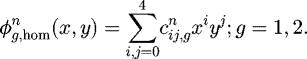 (1)
(1)
The coefficients of this expansion are determined by using the values of the average nodal fluxes determined with the coarse mesh nodal method. In 1985, Koebke and Hetzel [5] used a polynomial expansion, according to equation (1), in order to characterize the fast flux (g = 1), and a hyperbolic function expansion for the thermal flux (g = 2).
with  and
and  , h being the width of the fuel element.
Rempe et al. [6] also used polynomial expansions to determine the homogeneous distribution of fast neutron flux equation (1) and hyperbolic functions to represent the homogeneous distribution of thermal neutron flux. However, with a different approach than Koebke and Hetzelt [5] for the first term expansion,
Recently, Pessoa and Martinez [3] represented the pin to pin flux by a fourth-order expansion with a two-dimensional axial leakage treatment, so that diffusion equation can be solved analytically. This solution is a sum of a particular solution of the non-homogeneous equation and the general solution of the homogeneous differential equation. The boundary conditions are the four-total current on the surfaces of the node and four average fluxes in the node corners. According to Pessoa and Martinez [3], the larger errors occur in assemblies near baffle–reflector interfaces. One of the reasons pointed out there is that in the nuclear data generation for these assemblies resulted in important information being lost. Errors can be as large as 14.6% in those regions.
It is apparent from this discussion that flux reconstruction techniques are kind of an art, since there is no sound basis for choosing the flux form to be used. This has motivated investigating the use of techniques employing Artificial Intelligence (AI), which could be trained with real data, hoping to find smaller errors than in the literature. From the techniques available, we decided to exploit the SVR algorithm, of which a brief description follows.
The SV algorithm is a generalization of the algorithm developed by Vapnik and Lerner [7] in 1963 and Vapnik and Chervonenkis [8] in 1964. In the following years, Vapnik [2] continued to develop the technique that is characterized by statistical learning or VC theory. First, these algorithms were applied to classification problems. Currently, in addition to classification, the theory was extended to regression problems. The support vectors regression technique was applied to predict time series by Müller et al. [9] Drucker et al. [10] and Mattera and Haykin [11] in the late 1990s.
3 Support vectors regression (SVR)
Support vectors regression presents the principle of structural risk minimization, which considers the minimization of the upper limit of the generalization error [12]. The expected risk is defined as a function of the empirical risk, R
emp, which measures the error rate in a training set for a number of finite and fixed observations of the problem: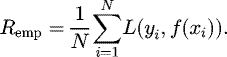 (2)
(2)
In equation (2), N is the number of points in the training set and L (xi
, f (xi
)) is the loss function, assumed quadratic in this work:
Thus, the L loss function corresponds, in our problem, to the difference between a target neutron flux and the estimated one. Moreover, the expected risk R emp corresponds to the average error of the estimated neutron flux. Hence, higher values of R emp means higher error and consequently higher risk of poor estimation of neutron fluxes.
Considering that we are looking for linear functions that relate the input data x
i
to the desired values y
i
through f (xi
) = w · xi
+ b, with b ∊ R and w ∊ X, where w · x
i
is the inner product in space X, the expected risk equation for N training samples is (3)
(3)
The structural risk minimization was proposed by Vapnik et al. [13] and it consists of reducing the value on the right of equation (3) in order to obtain the smallest expected risk. The SVR attempts to find the function f which relates the values x
i
to the values yi
, with a maximum deviation ε for the training data. Therefore, a space is created where all points with acceptable errors are within the interval [yi
− ε, yi
+ ε]. The SVR focuses on minimizing the second term of equation (6) such that the problem is to determine: subject to
Equation (3) does not take into account the results outside the range set by the choice of ε.
For the points outside this range to be considered, slack variables ξ and ξ* are introduced into the optimization problem.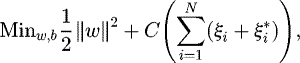
subject to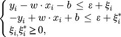
where C is a constant to be chosen and determines the trade-off among f and points xi
with errors greater than ε. The choice of C implies in determining w, which minimizes the slack variables. A loss function is used in this work to characterize the points outside ε, the ε-insensitive loss function, defined by equation (4):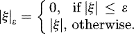 (4)
(4)
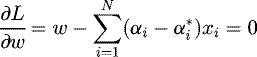
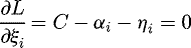
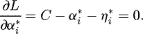
This primal optimization problem is difficult due to the inequalities in the constraints equations. Therefore, a dual problem is developed as an easier alternative to solve the optimization problem. This transformation from primal to dual problem considers a Lagrangian function having Lagrange multipliers as dual variables for each constraint of the primal problem. The dual problem Lagrangian function is given by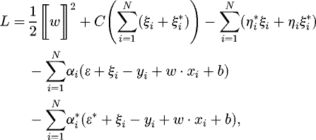 (5)where αi, αi, ηi
*, η*
i
are Lagrange multipliers restricted to be ≤0. Then, the problem becomes a problem of maximizing dual variables. On the other hand, the Lagrange function L will be minimized by deriving it with respect to each primal variable and equating these derivatives to zero:
(5)where αi, αi, ηi
*, η*
i
are Lagrange multipliers restricted to be ≤0. Then, the problem becomes a problem of maximizing dual variables. On the other hand, the Lagrange function L will be minimized by deriving it with respect to each primal variable and equating these derivatives to zero: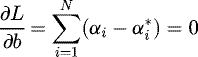 (6)
(6)
 (7)
(7)
 (8)
(8)
 (9)
(9)
Substituting equations (6)–(9) in equation (5), we have the dual problem as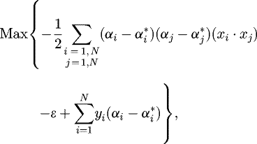 (10)
subject to
(10)
subject to  .
.
From equation (7), it can be seen that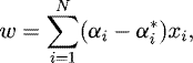
which determines f
(x) as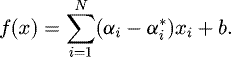
Therefore, to determine f, it is not necessary to determine w, which is a primal variable. Lagrange multipliers are obtained from the dual problem. The Karush–Kuhn–Tucker (KKT) conditions are used to interact between primal and dual problems as follows: (11)
(11)
 (12)
(12)
Equations (11) and (12) establish the first complementary KKT condition, where the dual variables α
i
and  are different from zero when
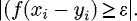 (13)
(13)
From equation (13), it can be concluded that it is not necessary to use all points x
i
to determine w but only those that make α
i
and  greater than zero. These points are the so-called support vectors [14].
To calculate b, the complementary KKT conditions are used with (14)
(14)
 (15)
(15)
Since α
i
and  in equations (14) and (15) must be different from zero, it results that the slack variables must be equal to zero. Thus, b can be determined by taking the points where Lagrangian multipliers vary on the interval (0, C). Now using equations (11) and (12), we get
Now, define a kernel function
Substituting this kernel function into the dual problem equations 15, we have
subject to:  .
.
Function f will now be determined by making
And then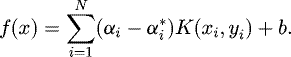
Finally, the kernel function used in this work is the radial basis function (RBF) presented below: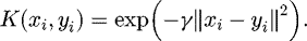
4 Application of SVR methodology to pin to pin flux reconstruction for a PWR nuclear reactor
The reactor studied in this work is a PWR reactor similar to Angra-1. This reactor has 121 (Fig. 1) 20 × 20 cm fuel elements of 3.60 m height, set in a 16 × 16 array (Fig. 2). Each element contains 256 pins distributed among nuclear fuel, burnable poison, water holes, etc. The fuel element nuclear parameters were homogenized, and the reactor was discretized using 20 × 20 × 20 cm nodes, totaling 1936 nodes: 121 nodes in x- and y-directions with 16 layers in the z-direction. These data are important for the nodal calculation with NEM. The nodes corresponding to lower and upper reflectors were discarded because they do not contribute to power generation.
4.1 Fundamental problem
NEM is applied to this discretized space in order to determine average values for fluxes and currents. In this process, as said earlier, the heterogeneity of information is lost, since NEM makes use of node homogenized cross sections. However, it is important for fuel cycle design and for safety reasons that pin to pin fluxes in every fuel element be determined for the whole core. Then, considering the average nodal flux values, total currents and partial fluxes at each face of the node, determined by NEM, which are input data for the SVR technique, one can obtain pin to pin neutron fluxes (representing the target data) in each of the 256 pins constituents of the fuel assembly. This study has focused on obtaining the thermal flux pin values, since the same procedure can be performed for the fast group. Therefore, from this point on, the ϕ g,hom(x, y) shall be referred to as ϕ hom(x, y).
To determine the optimal values for the parameter C, the penalty factor, and γ, a parameter of the RBF kernel function, the learning process was attained through an automatic search process [12]. The training and validation sets were divided into a proportion of 70–30% for training and validation purposes, using the multifold-cross-validation technique. After the learning process was done, the algorithm could use the pair (C, γ) for reconstruction purposes.
The data were processed according to the normalization: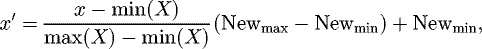 where x is a vector space X and Newmax and Newmin are chosen according to the purpose. In this work, the new range will be between [−1, 1]. The reference values for the pin fluxes were obtained from NEM, with a fine spatial discretization mesh, with dimensions on the order of the fuel rod size.
4.2 Methodology
First, the reconstruction of the pin to pin flux was done for two fuel rods, pin 01 and pin 170, in fuel assembly 01, as shown in Figures 1 and 2. Then, for a first test, one fuel element was removed for testing. Thus, a total of 120 sample fuel assemblies were available for training and validation purposes, with each instance containing a vector entry of order [16 × 19], because each instance has the values of the 16 fuel assembly layer divisions. Each example was correlated with 16 values of the pin to pin flux, one for each layer. So, for the test, a set of [16 × 19] was presented to the algorithm and the output was a vector of [16 × 1], regarding the neutron flux values at pin 01 of the element 01. It will be shown in Section 4.1 that determining a value for C and γ parameters to reconstruct the flux pin to pin for a complete fuel rod, at a given time, is not efficient. To solve this problem, we presented 16 pairs (C, γ) for the algorithm, one pair for each layer.
To examine the new methodology of training/validation and testing, all data from two selected fuel elements were removed, the first near the side reflector, fuel element 53, and the second near the center of the reactor configuration, 87. The reconstruction was carried out for fuel element 53, but with a pair (C, γ) for each pin layer. This was taken into consideration because it was found that for a given fuel element, the values of the pin to pin fluxes for each layer do not present large variations (Fig. 3).
Finally, the reconstruction for fuel element 87 was performed using the same parameters used to reconstruct the fluxes for fuel element 53. Equation (8) shows the calculation of the error (e), where  is the pin flux determined by the algorithm and (ϕ
hom,R
(x, y)) is the neutron flux in the reference pin, that is, the one obtained with fine mesh NEM discretization. For the training error, we have chosen the maximum value of 0.001% and for validation, a maximum error of 0.01%.
is the pin flux determined by the algorithm and (ϕ
hom,R
(x, y)) is the neutron flux in the reference pin, that is, the one obtained with fine mesh NEM discretization. For the training error, we have chosen the maximum value of 0.001% and for validation, a maximum error of 0.01%.
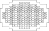 |
Fig. 1 Core configuration. |
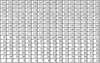 |
Fig. 2 Fuel assembly pin identification. |
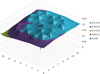 |
Fig. 3 Pin to pin flux distribution for assembly 53 on the first layer. |
5 Analysis of results
5.1 Reconstruction for two fuel rods using the same parameters of learning
Figure 4 shows the results obtained for pin 01 of the fuel assembly 01. The training and validation algorithms were performed taking as the target the value of pin number 01 for all fuel assemblies. After the training and validation, the algorithm found the optimum pair (C, γ) for reconstruction of pin 01 flux of fuel assembly 01. Figure 4 shows that the algorithm obtained a 1.17% error in layer 8 for the pin flux. The same learning parameters for the reconstruction of the flux pin to pin 170 were used.
The differences between the reference fluxes and the predicted fluxes are larger for pin 170, as shown in Figure 5, with a maximum error of 1.3% in layer 3. This is because the same parameters used to estimate the flux of pin 01 were used for pin 170. This result makes clear that each pin has its specificity, and the optimal parameters for a pin do not necessarily apply to others.
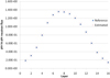 |
Fig. 4 Comparison of the pin to pin reference fluxes and those estimated by the algorithm for pin 01 of assembly 01. |
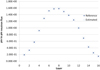 |
Fig. 5 Comparison of the pin to pin of reference fluxes and those estimated by the algorithm for pin 170 of assembly 01. |
5.2 Neutron flux pin to pin reconstruction for two elements
This time, two fuel elements were removed from the training and validation sets. The elements removed for the test were elements 53 and 87, according to Figure 1. Analyzing the first layer element 01 (Fig. 3), it can be seen that the pin to pin neutron fluxes do not have wide variations. The average is given by 0.198584 cm−2 s−1 and variance and standard deviation are, respectively, 0.000706 and 0.026584. With these observations, a new approach to input data for the training and validation methods was performed. Input data were divided into 16 layers. So, at this point, an array with the pairs (C, γ) was generated for each node for each layer.
Figure 6 shows the results for predicted values for the neutron fluxes in the first layer, assembly 53, which has been submitted to the training and validation algorithm. As can be seen, the maximum error obtained is 1.29%, according to equation (8). Recall that the fuel assemblies are surrounded by the side reflector of the reactor, which according to Pessoa and Martinez [3] is the most critical part of the reconstruction.
Figure 7 shows the reconstruction of the pin to pin fluxes for assembly 53. It also shows the ratio between the maximum and the average pin to pin fluxes, with a maximum of 1.76% error.
Table 1 shows the maximum values of errors obtained, according to equation (8), the distribution of neutrons by layers of all the pins 256 of assembly 53.
Figure 8 shows the comparison between the values obtained from the ratio between maximum and average flux value of the same pin. The comparison shows a maximum error of 1.27% for the 256 pins in assembly 87, using the same learning parameters to determine the pin to pin fluxes in assembly 53.
The computational time for the search of the optimal parameters of learning, with respect to training and validation procedures is very large, about 72 h. However, with the optimal parameters defined, the algorithm provides the values of the pin to pin fluxes for each test fuel assembly in negligible time.
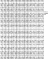 |
Fig. 6 Comparing the reference to estimated fluxes by the algorithm, for each pin of the first layer of assembly 53. |
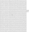 |
Fig. 7 Ratios between maximum and average values of the pin to pin fluxes for assembly 53. |
Maximum errors obtained for all layers of assembly 53.
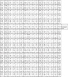 |
Fig. 8 Ratios between maximum and average values of the pin to pin fluxes for assembly 87. |
6 Conclusions
These results show that the machine learning technique using SVR is able to reconstruct the pin to pin fluxes. From the data of the first nuclear reactor cycle, the learning parameters can be determined. The search for optimal learning parameters takes a very large computational time, about 72 h. However, the prediction, once these parameters are found, is very quick. Pessoa and Martinez [3] found error exceeding 14% in pin to pin flux reconstruction for the assembly surrounding the baffle/reflector. For assembly 53, which surrounds the baffle/reflector, the maximum error obtained by the technique presented in this work was 1.76 %. A direct application of this work is that the machine learning using SVR can be incorporated into reactor physics codes. The SVR could work in parallel with reactor physics codes for the data in real time and determine pin to pin neutron fluxes for subsequent cycles in a nuclear reactor, that is, in fuel reload calculations. After this, the system is able to determine the safety factors, which depend on these fluxes, in a very small computational time for future cycles of a nuclear reactor power.
Author contribution statement
This paper was developed as a doctoral thesis theme, which I (A. Alvim) offered to Wanderson, to be developed under my supervision and also of Professor Fernando Carvalho da Silva, in the Reactor Physics area of the Nuclear Engineering Programme of COPPE/UFRJ. Professor Fernando and I have worked previously in flux reconstruction problems with the methods described in the review section of the paper. Professor Leandro Guimarães Marques Alvim, of UFFRJ, has provided assistance to Wanderson with respect to the SVM method in relation to the flux reconstruction problem, which is one of his areas of expertise.
All the authors have contributed with analyses and critical judgement of results obtained in the course of the work. All the authors have reviewed technically the paper and I was in charge, as corresponding author, of incorporating the referees' requirements and of the writing of the entire paragraph detailing the SVM method.
References
- H. Finnemann, F. Bennewitz, M.R. Wagner, Interface current techniques for multidimensional reactor calculations, Atomkernenergie 300 , 123 (1977) [Google Scholar]
- V.N. Vapnik, The Nature of Statistical Learning Theory , 2nd edn. (Springer, New York, 1999) [Google Scholar]
- P.O. Pessoa, A.S. Martinez, Methods for reconstruction of the density distribution of nuclear power, Ann. Nucl. Energy 83 , 76 (2015) [CrossRef] [Google Scholar]
- K. Koebke, M.R. Wagner, The determination of the pin power distribution in a reactor core on the basis of coarse mesh methods, Atomkernenergie 30 , 136 (1977) [Google Scholar]
- K. Koebke, L. Helzelt, On the reconstruction of local homogeneous neutron flux and current distributions of light water reactor nodal schemes, Nucl. Sci. Eng. 91 , 123 (1985) [CrossRef] [Google Scholar]
- K.R. Rempe, K.S. Smith, A.F. Henry, SIMULATE-3 pin power reconstruction: methodology and benchmarking, Nucl. Sci. Eng. 103 , 334 (1989) [CrossRef] [Google Scholar]
- V. Vapnik, A. Lerner, Pattern recognition using generalized portrait method, Autom. Remote Control 24 , 774 (1963) [Google Scholar]
- V. Vapnik, A. Chervonenkis, A note on one class of perceptrons, Autom. Remote Control 25 , 103 (1964) [Google Scholar]
- K.R. Müller, A. Smola, G. Rätsch, B. Schölkopf, J. Kohlmorgen, V. Vapnik, Predicting time series with support vector machine, in Artificial Neural Networks – ICANN'97, Springer Lecture Notes in Computer Science, edited by W. Gerstner, A. Germond, M. Hasler, J.-D. Nicoud (Springer, Berlin, 1997), Vol. 1327, pp. 999−1004 [Google Scholar]
- H. Drucker, C.J.C. Burges, L. Kaufman, A. Smola, V. Vapnik, Support vector regression machines, in Advances in Neural Information Processing Systems 9, edited by M. Mozer, M. Jordan, T. Petsche (MIT Press, Cambridge, MA), pp. 155–161 [Google Scholar]
- D. Mattera, S. Haykin, Support vector machine for dynamic reconstruction of a chaotic system, in Advances in Kernel Methods − Support Vector Learning , edited by B. Shölkopf, C.J.C. Burgues, A.J. Smola (MIT Press, Cambridge, MA, 1999), pp. 211–242 [Google Scholar]
- F. Pedrogosa, G. Varoquaux, A. Gramfort, V. Michel, B. Thirion, O. Grisel, M. Blondel, P. Prettenhofer, R. Weiss, V. Dubourg, J. Vanderplas, A. Passos, D. Cournapeau, M. Brucher, M. Perrot, E. Duchesnay, Scikit-learn: machine learning in Python, J. Mach. Learn. Res. 12 , 2825 (2011) [Google Scholar]
- V. Vapnik, S. Golowich, A. Smola, Support vector method for function approximation, regression estimation, and signal processing, in Neural Information Processing Systems , edited by M. Mozer, M. Jordan, T. Petsche (MIT Press, Cambridge, MA, 1997), Vol. 9 [Google Scholar]
- A.J. Smola, B. Schölkopf, A Tutorial on Support Vector Regression, Royal Holloway College, NeuroColt Technical Report (NC-TR-98-030), University of London, UK, 1998 [Google Scholar]
Cite this article as: W.F.P. Neto, A.C.M. Alvim, F.C. Silva, L.G.M. Alvim, Pin to pin neutron flux reconstruction in a PWR reactor using support vector regression (SVR) technique, EPJ Nuclear Sci. Technol. 5, 3 (2019)
All Tables
All Figures
|
Fig. 1 Core configuration. |
| In the text | |
|
Fig. 2 Fuel assembly pin identification. |
| In the text | |
|
Fig. 3 Pin to pin flux distribution for assembly 53 on the first layer. |
| In the text | |
|
Fig. 4 Comparison of the pin to pin reference fluxes and those estimated by the algorithm for pin 01 of assembly 01. |
| In the text | |
|
Fig. 5 Comparison of the pin to pin of reference fluxes and those estimated by the algorithm for pin 170 of assembly 01. |
| In the text | |
|
Fig. 6 Comparing the reference to estimated fluxes by the algorithm, for each pin of the first layer of assembly 53. |
| In the text | |
|
Fig. 7 Ratios between maximum and average values of the pin to pin fluxes for assembly 53. |
| In the text | |
|
Fig. 8 Ratios between maximum and average values of the pin to pin fluxes for assembly 87. |
| In the text | |
Current usage metrics show cumulative count of Article Views (full-text article views including HTML views, PDF and ePub downloads, according to the available data) and Abstracts Views on Vision4Press platform.
Data correspond to usage on the plateform after 2015. The current usage metrics is available 48-96 hours after online publication and is updated daily on week days.
Initial download of the metrics may take a while.